Flight dynamics (fixed-wing aircraft)
This article's lead section may not adequately summarize its contents. (July 2018) |

Flight dynamics is the science of air vehicle orientation and control in three dimensions. The three critical flight dynamics parameters are the angles of rotation in three dimensions about the vehicle's center of mass, known as pitch, roll and yaw.
Aerospace engineers develop control systems for a vehicle's orientation (attitude) about its center of mass. The control systems include actuators, which exert forces in various directions, and generate rotational forces or moments about the aerodynamic center of the aircraft, and thus rotate the aircraft in pitch, roll, or yaw. For example, a pitching moment is a vertical force applied at a distance forward or aft from the aerodynamic center of the aircraft, causing the aircraft to pitch up or down.
Roll, pitch and yaw refer to rotations about the respective axes starting from a defined steady flight equilibrium state. The equilibrium roll angle is known as wings level or zero bank angle, equivalent to a level heeling angle on a ship. Yaw is known as "heading". The equilibrium pitch angle in submarine and airship parlance is known as "trim", but in aircraft, "trim" usually refers to the equilibrium angle of attack, rather than orientation. However, common usage ignores this distinction between equilibrium and dynamic cases.
The most common aeronautical convention defines the roll as acting about the longitudinal axis, positive with the starboard (right) wing down. The yaw is about the vertical body axis, positive with the nose to starboard. Pitch is about an axis perpendicular to the longitudinal plane of symmetry, positive nose up.[citation needed]
A fixed-wing aircraft increases or decreases the lift generated by the wings when it pitches nose up or down by increasing or decreasing the angle of attack (AOA). The roll angle is also known as bank angle on a fixed-wing aircraft, which usually "banks" to change the horizontal direction of flight. An aircraft is usually streamlined from nose to tail to reduce drag making it typically advantageous to keep the sideslip angle near zero, though there are instances when an aircraft may be deliberately "sideslipped" for example a slip in a fixed-wing aircraft.[citation needed]
@media all and (max-width:720px){.mw-parser-output .tmulti>.thumbinner{width:100%!important;max-width:none!important}.mw-parser-output .tmulti .tsingle{float:none!important;max-width:none!important;width:100%!important;text-align:center}}


yaw or heading angle definition[1]

pitch angle definition[1]

Contents
1 Introduction
1.1 Reference frames
1.2 Design cases
2 Forces of flight
2.1 Aerodynamic force
2.1.1 Components of the aerodynamic force
2.1.2 Aerodynamic coefficients
2.1.3 Dimensionless parameters and aerodynamic regimes
2.1.4 Drag coefficient equation and aerodynamic efficiency
2.1.5 Parabolic and generic drag coefficient
2.1.6 Variation of parameters with the Mach number
2.1.7 Aerodynamic force in a specified atmosphere
2.2 Features and selection of the propeller
3 Static stability and control
3.1 Longitudinal static stability
3.2 Directional stability
4 Dynamic stability and control
4.1 Longitudinal modes
4.1.1 Short-period pitch oscillation
4.1.2 Phugoid
4.2 Lateral modes
4.2.1 Dutch roll
4.2.2 Lateral and longitudinal stability derivatives
4.2.3 Equations of motion
4.2.4 Roll subsidence
4.2.5 Spiral mode
4.2.5.1 Spiral mode trajectory
5 See also
6 References
6.1 Notes
6.2 Bibliography
7 External links
Introduction
Reference frames
Three right-handed, Cartesian coordinate systems see frequent use in flight dynamics. The first coordinate system has an origin fixed in the reference frame of the Earth:
- Earth frame
- Origin - arbitrary, fixed relative to the surface of the Earth
xE axis - positive in the direction of north
yE axis - positive in the direction of east
zE axis - positive towards the center of the Earth
In many flight dynamics applications, the Earth frame is assumed to be inertial with a flat xE,yE-plane, though the Earth frame can also be considered a spherical coordinate system with origin at the center of the Earth.
The other two reference frames are body-fixed, with origins moving along with the aircraft, typically at the center of gravity. For an aircraft that is symmetric from right-to-left, the frames can be defined as:
- Body frame
- Origin - airplane center of gravity
xb axis - positive out the nose of the aircraft in the plane of symmetry of the aircraft
zb axis - perpendicular to the xb axis, in the plane of symmetry of the aircraft, positive below the aircraft
yb axis - perpendicular to the xb,zb-plane, positive determined by the right-hand rule (generally, positive out the right wing)
- Wind frame
- Origin - airplane center of gravity
xw axis - positive in the direction of the velocity vector of the aircraft relative to the air
zw axis - perpendicular to the xw axis, in the plane of symmetry of the aircraft, positive below the aircraft
yw axis - perpendicular to the xw,zw-plane, positive determined by the right hand rule (generally, positive to the right)
Asymmetric aircraft have analogous body-fixed frames, but different conventions must be used to choose the precise directions of the x and z axes.
The Earth frame is a convenient frame to express aircraft translational and rotational kinematics. The Earth frame is also useful in that, under certain assumptions, it can be approximated as inertial. Additionally, one force acting on the aircraft, weight, is fixed in the +zE direction.
The body frame is often of interest because the origin and the axes remain fixed relative to the aircraft. This means that the relative orientation of the Earth and body frames describes the aircraft attitude. Also, the direction of the force of thrust is generally fixed in the body frame, though some aircraft can vary this direction, for example by thrust vectoring.
The wind frame is a convenient frame to express the aerodynamic forces and moments acting on an aircraft. In particular, the net aerodynamic force can be divided into components along the wind frame axes, with the drag force in the −xw direction and the lift force in the −zw direction.
In addition to defining the reference frames, the relative orientation of the reference frames can be determined. The relative orientation can be expressed in a variety of forms, including:
- Direction cosine or rotation matrices
- Euler angles
- Quaternions
The various Euler angles relating the three reference frames are important to flight dynamics. Many Euler angle conventions exist, but all of the rotation sequences presented below use the z-y'-x" convention. This convention corresponds to a type of Tait-Bryan angles, which are commonly referred to as Euler angles. This convention is described in detail below for the roll, pitch, and yaw Euler angles that describe the body frame orientation relative to the Earth frame. The other sets of Euler angles are described below by analogy.
To transform from the Earth frame to the body frame using Euler angles, the following rotations are done in the order prescribed. First, rotate the Earth frame axes xE and yE around the zE axis by the yaw angle ψ. This results in an intermediate reference frame with axes denoted x',y',z', where z'=zE. Second, rotate the x' and z' axes around the y' axis by the pitch angle θ. This results in another intermediate reference frame with axes denoted x",y",z", where y"=y'. Finally, rotate the y" and z" axes around the x" axis by the roll angle φ. The reference frame that results after the three rotations is the body frame.
Based on the rotations and axes conventions above, the yaw angle ψ is the angle between north and the projection of the aircraft longitudinal axis onto the horizontal plane, the pitch angle θ is the angle between the aircraft longitudinal axis and horizontal, and the roll angle φ represents a rotation around the aircraft longitudinal axis after rotating by yaw and pitch.
To transform from the Earth frame to the wind frame, the three Euler angles are the bank angle μ, the flight path angle γ, and the heading angle σ. When performing the rotations described above to obtain the wind frame from the Earth frame, (μ,γ,σ) are analogous to (φ,θ,ψ), respectively. The heading angle σ is the angle between north and the horizontal component of the velocity vector, which describes which direction the aircraft is moving relative to cardinal directions. The flight path angle γ is the angle between horizontal and the velocity vector, which describes whether the aircraft is climbing or descending. The bank angle μ represents a rotation of the lift force around the velocity vector, which may indicate whether the airplane is turning.
To transform from the wind frame to the body frame, the two Euler angles are the angle of attack α and the sideslip angle β. When performing the rotations described earlier to obtain the body frame from the wind frame, (α,β) are analogous to (θ,ψ), respectively; the angle analogous to φ in this transformation is always zero. The sideslip angle β is the angle between the velocity vector and the projection of the aircraft longitudinal axis onto the xw,yw-plane, which describes whether there is a lateral component to the aircraft velocity, also known as sideslip. The angle of attack α is the angle between the xw,yw-plane and the aircraft longitudinal axis and, among other things, is an important variable in determining the magnitude of the force of lift.
Design cases
In analyzing the stability of an aircraft, it is usual to consider perturbations about a nominal steady flight state. So the analysis would be applied, for example, assuming:
- Straight and level flight
- Turn at constant speed
- Approach and landing
- Takeoff
The speed, height and trim angle of attack are different for each flight condition, in addition, the aircraft will be configured differently, e.g. at low speed flaps may be deployed and the undercarriage may be down.
Except for asymmetric designs (or symmetric designs at significant sideslip), the longitudinal equations of motion (involving pitch and lift forces) may be treated independently of the lateral motion (involving roll and yaw).
The following considers perturbations about a nominal straight and level flight path.
To keep the analysis (relatively) simple, the control surfaces are assumed fixed throughout the motion, this is stick-fixed stability. Stick-free analysis requires the further complication of taking the motion of the control surfaces into account.
Furthermore, the flight is assumed to take place in still air, and the aircraft is treated as a rigid body.
Forces of flight
Three forces act on an aircraft in flight: weight, thrust, and the aerodynamic force.
Aerodynamic force
Components of the aerodynamic force
The expression to calculate the aerodynamic force is:
- FA=∫Σ(−Δpn+f)dσ{displaystyle mathbf {F} _{A}=int _{Sigma }(-Delta pmathbf {n} +mathbf {f} ),dsigma }
- FA=∫Σ(−Δpn+f)dσ{displaystyle mathbf {F} _{A}=int _{Sigma }(-Delta pmathbf {n} +mathbf {f} ),dsigma }

where:
Δp≡{displaystyle Delta pequiv }Difference between static pressure and free current pressure
n≡{displaystyle mathbf {n} equiv }outer normal vector of the element of area
f≡{displaystyle mathbf {f} equiv }tangential stress vector practised by the air on the body
Σ≡{displaystyle Sigma equiv }adequate reference surface
projected on wind axes we obtain:
- FA=−(iwD+jwQ+kwL){displaystyle mathbf {F} _{A}=-(mathbf {i} _{w}D+mathbf {j} _{w}Q+mathbf {k} _{w}L)}
- FA=−(iwD+jwQ+kwL){displaystyle mathbf {F} _{A}=-(mathbf {i} _{w}D+mathbf {j} _{w}Q+mathbf {k} _{w}L)}

where:
D≡{displaystyle Dequiv }Drag
Q≡{displaystyle Qequiv }Lateral force
L≡{displaystyle Lequiv }Lift
Aerodynamic coefficients
Dynamic pressure of the free current ≡q=12ρV2{displaystyle equiv q={tfrac {1}{2}},rho ,V^{2}}

Proper reference surface (wing surface, in case of planes) ≡S{displaystyle equiv S}

Pressure coefficient ≡Cp=p−p∞q{displaystyle equiv C_{p}={dfrac {p-p_{infty }}{q}}}

Friction coefficient ≡Cf=fq{displaystyle equiv C_{f}={dfrac {f}{q}}}

Drag coefficient ≡Cd=DqS=−1S∫Σ[(−Cp)n∙iw+Cft∙iw]dσ{displaystyle equiv C_{d}={dfrac {D}{qS}}=-{dfrac {1}{S}}int _{Sigma }[(-C_{p})mathbf {n} bullet mathbf {i_{w}} +C_{f}mathbf {t} bullet mathbf {i_{w}} ],dsigma }
![equiv C_{d}={dfrac {D}{qS}}=-{dfrac {1}{S}}int _{Sigma }[(-C_{p}){mathbf {n}}bullet {mathbf {i_{w}}}+C_{f}{mathbf {t}}bullet {mathbf {i_{w}}}],dsigma](https://wikimedia.org/api/rest_v1/media/math/render/svg/b16598ab4310bdfb79e62c3b3ffa8fb3d7356bea)
Lateral force coefficient ≡CQ=QqS=−1S∫Σ[(−Cp)n∙jw+Cft∙jw]dσ{displaystyle equiv C_{Q}={dfrac {Q}{qS}}=-{dfrac {1}{S}}int _{Sigma }[(-C_{p})mathbf {n} bullet mathbf {j_{w}} +C_{f}mathbf {t} bullet mathbf {j_{w}} ],dsigma }
![equiv C_{Q}={dfrac {Q}{qS}}=-{dfrac {1}{S}}int _{Sigma }[(-C_{p}){mathbf {n}}bullet {mathbf {j_{w}}}+C_{f}{mathbf {t}}bullet {mathbf {j_{w}}}],dsigma](https://wikimedia.org/api/rest_v1/media/math/render/svg/058ae7bf706024c1943fc8d36eb6ca9a35653039)
Lift coefficient ≡CL=LqS=−1S∫Σ[(−Cp)n∙kw+Cft∙kw]dσ{displaystyle equiv C_{L}={dfrac {L}{qS}}=-{dfrac {1}{S}}int _{Sigma }[(-C_{p})mathbf {n} bullet mathbf {k_{w}} +C_{f}mathbf {t} bullet mathbf {k_{w}} ],dsigma }
![equiv C_{L}={dfrac {L}{qS}}=-{dfrac {1}{S}}int _{Sigma }[(-C_{p}){mathbf {n}}bullet {mathbf {k_{w}}}+C_{f}{mathbf {t}}bullet {mathbf {k_{w}}}],dsigma](https://wikimedia.org/api/rest_v1/media/math/render/svg/a92e802e0eb8cad0e69f7849d35e2b6dbec96a1b)
It is necessary to know Cp and Cf in every point on the considered surface.
Dimensionless parameters and aerodynamic regimes
In absence of thermal effects, there are three remarkable dimensionless numbers:
- Compressibility of the flow:
Mach number ≡M=Va{displaystyle equiv M={dfrac {V}{a}}}

- Viscosity of the flow:
Reynolds number ≡Re=ρVlμ{displaystyle equiv Re={dfrac {rho Vl}{mu }}}

- Rarefaction of the flow:
Knudsen number ≡Kn=λl{displaystyle equiv Kn={dfrac {lambda }{l}}}

where:
a=kRθ≡{displaystyle a={sqrt {kRtheta }}equiv }speed of sound
R≡{displaystyle Requiv }gas constant by mass unity
θ≡{displaystyle theta equiv }absolute temperature
λ=μρπ2Rθ=MRekπ2≡{displaystyle lambda ={dfrac {mu }{rho }}{sqrt {dfrac {pi }{2Rtheta }}}={dfrac {M}{Re}}{sqrt {dfrac {kpi }{2}}}equiv }mean free path
According to λ there are three possible rarefaction grades and their corresponding motions are called:
- Continuum current (negligible rarefaction): MRe≪1{displaystyle {dfrac {M}{Re}}ll 1}
- Transition current (moderate rarefaction): MRe≈1{displaystyle {dfrac {M}{Re}}approx 1}
- Free molecular current (high rarefaction): MRe≫1{displaystyle {dfrac {M}{Re}}gg 1}


The motion of a body through a flow is considered, in flight dynamics, as continuum current. In the outer layer of the space that surrounds the body viscosity will be negligible. However viscosity effects will have to be considered when analysing the flow in the nearness of the boundary layer.
Depending on the compressibility of the flow, different kinds of currents can be considered:
Incompressible subsonic current: 0<M<0.3{displaystyle 0<M<0.3}
Compressible subsonic current: 0.3<M<0.8{displaystyle 0.3<M<0.8}
Transonic current: 0.8<M<1.2{displaystyle 0.8<M<1.2}
Supersonic current: 1.2<M<5{displaystyle 1.2<M<5}
Hypersonic current: 5<M{displaystyle 5<M}


Drag coefficient equation and aerodynamic efficiency
If the geometry of the body is fixed and in case of symmetric flight (β=0 and Q=0), pressure and friction coefficients are functions depending on:
- Cp=Cp(α,M,Re,P){displaystyle C_{p}=C_{p}(alpha ,M,Re,P)}
- Cf=Cf(α,M,Re,P){displaystyle C_{f}=C_{f}(alpha ,M,Re,P)}
- Cp=Cp(α,M,Re,P){displaystyle C_{p}=C_{p}(alpha ,M,Re,P)}


where:
α≡{displaystyle alpha equiv }angle of attack
P≡{displaystyle Pequiv }considered point of the surface
Under these conditions, drag and lift coefficient are functions depending exclusively on the angle of attack of the body and Mach and Reynolds numbers. Aerodynamic efficiency, defined as the relation between lift and drag coefficients, will depend on those parameters as well.
- {CD=CD(α,M,Re)CL=CL(α,M,Re)E=E(α,M,Re)=CLCD{displaystyle {begin{cases}C_{D}=C_{D}(alpha ,M,Re)\C_{L}=C_{L}(alpha ,M,Re)\E=E(alpha ,M,Re)={dfrac {C_{L}}{C_{D}}}\end{cases}}}
- {CD=CD(α,M,Re)CL=CL(α,M,Re)E=E(α,M,Re)=CLCD{displaystyle {begin{cases}C_{D}=C_{D}(alpha ,M,Re)\C_{L}=C_{L}(alpha ,M,Re)\E=E(alpha ,M,Re)={dfrac {C_{L}}{C_{D}}}\end{cases}}}

It is also possible to get the dependency of the drag coefficient respect to the lift coefficient. This relation is known as the drag coefficient equation:
CD=CD(CL,M,Re)≡{displaystyle C_{D}=C_{D}(C_{L},M,Re)equiv }drag coefficient equation
The aerodynamic efficiency has a maximum value, Emax, respect to CL where the tangent line from the coordinate origin touches the drag coefficient equation plot.
The drag coefficient, CD, can be decomposed in two ways. First typical decomposition separates pressure and friction effects:
- CD=CDf+CDp{CDf=DqS=−1S∫ΣCft∙iwdσCDp=DqS=−1S∫Σ(−Cp)n∙iwdσ{displaystyle C_{D}=C_{Df}+C_{Dp}{begin{cases}C_{Df}={dfrac {D}{qS}}=-{dfrac {1}{S}}int _{Sigma }C_{f}mathbf {t} bullet mathbf {i_{w}} ,dsigma \C_{Dp}={dfrac {D}{qS}}=-{dfrac {1}{S}}int _{Sigma }(-C_{p})mathbf {n} bullet mathbf {i_{w}} ,dsigma end{cases}}}
- CD=CDf+CDp{CDf=DqS=−1S∫ΣCft∙iwdσCDp=DqS=−1S∫Σ(−Cp)n∙iwdσ{displaystyle C_{D}=C_{Df}+C_{Dp}{begin{cases}C_{Df}={dfrac {D}{qS}}=-{dfrac {1}{S}}int _{Sigma }C_{f}mathbf {t} bullet mathbf {i_{w}} ,dsigma \C_{Dp}={dfrac {D}{qS}}=-{dfrac {1}{S}}int _{Sigma }(-C_{p})mathbf {n} bullet mathbf {i_{w}} ,dsigma end{cases}}}

There's a second typical decomposition taking into account the definition of the drag coefficient equation. This decomposition separates the effect of the lift coefficient in the equation, obtaining two terms CD0 and CDi. CD0 is known as the parasitic drag coefficient and it is the base draft coefficient at zero lift. CDi is known as the induced drag coefficient and it is produced by the body lift.
- CD=CD0+CDi{CD0=(CD)CL=0CDi{displaystyle C_{D}=C_{D0}+C_{Di}{begin{cases}C_{D0}=(C_{D})_{C_{L}=0}\C_{Di}end{cases}}}
- CD=CD0+CDi{CD0=(CD)CL=0CDi{displaystyle C_{D}=C_{D0}+C_{Di}{begin{cases}C_{D0}=(C_{D})_{C_{L}=0}\C_{Di}end{cases}}}

Parabolic and generic drag coefficient
A good attempt for the induced drag coefficient is to assume a parabolic dependency of the lift
- CDi=kCL2⇒CD=CD0+kCL2{displaystyle C_{Di}=kC_{L}^{2}Rightarrow C_{D}=C_{D0}+kC_{L}^{2}}

Aerodynamic efficiency is now calculated as:
- E=CLCD0+kCL2⇒{Emax=12kCD0(CL)Emax=CD0k(CDi)Emax=CD0{displaystyle E={dfrac {C_{L}}{C_{D0}+kC_{L}^{2}}}Rightarrow {begin{cases}E_{max}={dfrac {1}{2{sqrt {kC_{D0}}}}}\(C_{L})_{Emax}={sqrt {dfrac {C_{D0}}{k}}}\(C_{Di})_{Emax}=C_{D0}end{cases}}}

If the configuration of the plane is symmetrical respect to the XY plane, minimum drag coefficient equals to the parasitic drag of the plane.
- CDmin=(CD)CL=0=CD0{displaystyle C_{Dmin}=(C_{D})_{CL=0}=C_{D0}}

In case the configuration is asymmetrical respect to the XY plane, however, minimum flag differs from the parasitic drag. On these cases, a new approximate parabolic drag equation can be traced leaving the minimum drag value at zero lift value.
- CDmin=CDM≠(CD)CL=0{displaystyle C_{Dmin}=C_{DM}neq (C_{D})_{CL=0}}

- CD=CDM+k(CL−CLM)2{displaystyle C_{D}=C_{DM}+k(C_{L}-C_{LM})^{2}}

Variation of parameters with the Mach number
The Coefficient of pressure varies with Mach number by the relation given below:[2]
- Cp=Cp0|1−M∞2|{displaystyle C_{p}={frac {C_{p0}}{sqrt {|1-{M_{infty }}^{2}|}}}}
- Cp=Cp0|1−M∞2|{displaystyle C_{p}={frac {C_{p0}}{sqrt {|1-{M_{infty }}^{2}|}}}}

where
- Cp is the compressible pressure coefficient
- Cp0 is the incompressible pressure coefficient
M∞ is the freestream Mach number.
This relation is reasonably accurate for 0.3 < M < 0.7 and when M = 1 it becomes ∞ which is impossible physical situation and is called Prandtl–Glauert singularity.
Aerodynamic force in a specified atmosphere
see Aerodynamic force
Features and selection of the propeller
Static stability and control
Longitudinal static stability
see Longitudinal static stability
Directional stability
Directional or weathercock stability is concerned with the static stability of the airplane about the z axis. Just as in the case of longitudinal stability it is desirable that the aircraft should tend to return to an equilibrium condition when subjected to some form of yawing disturbance. For this the slope of the yawing moment curve must be positive.
An airplane possessing this mode of stability will always point towards the relative wind, hence the name weathercock stability.
Dynamic stability and control
Longitudinal modes
It is common practice to derive a fourth order characteristic equation to describe the longitudinal motion, and then factorize it approximately into a high frequency mode and a low frequency mode. The approach adopted here is using qualitative knowledge of aircraft behavior to simplify the equations from the outset, reaching the result by a more accessible route.
The two longitudinal motions (modes) are called the short period pitch oscillation (SPPO), and the phugoid.
Short-period pitch oscillation
A short input (in control systems terminology an impulse) in pitch (generally via the elevator in a standard configuration fixed-wing aircraft) will generally lead to overshoots about the trimmed condition. The transition is characterized by a damped simple harmonic motion about the new trim. There is very little change in the trajectory over the time it takes for the oscillation to damp out.
Generally this oscillation is high frequency (hence short period) and is damped over a period of a few seconds. A real-world example would involve a pilot selecting a new climb attitude, for example 5° nose up from the original attitude. A short, sharp pull back on the control column may be used, and will generally lead to oscillations about the new trim condition. If the oscillations are poorly damped the aircraft will take a long period of time to settle at the new condition, potentially leading to Pilot-induced oscillation. If the short period mode is unstable it will generally be impossible for the pilot to safely control the aircraft for any period of time.
This damped harmonic motion is called the short period pitch oscillation, it arises from the tendency of a stable aircraft to point in the general direction of flight. It is very similar in nature to the weathercock mode of missile or rocket configurations. The motion involves mainly the pitch attitude θ{displaystyle theta }


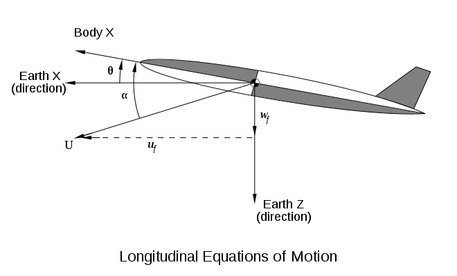
- uf=Ucos(θ−α){displaystyle u_{f}=Ucos(theta -alpha )}
- wf=Usin(θ−α){displaystyle w_{f}=Usin(theta -alpha )}
- uf=Ucos(θ−α){displaystyle u_{f}=Ucos(theta -alpha )}


where uf{displaystyle u_{f}}

- Xf=mdufdt=mdUdtcos(θ−α)−mUd(θ−α)dtsin(θ−α){displaystyle X_{f}=m{frac {du_{f}}{dt}}=m{frac {dU}{dt}}cos(theta -alpha )-mU{frac {d(theta -alpha )}{dt}}sin(theta -alpha )}
- Zf=mdwfdt=mdUdtsin(θ−α)+mUd(θ−α)dtcos(θ−α){displaystyle Z_{f}=m{frac {dw_{f}}{dt}}=m{frac {dU}{dt}}sin(theta -alpha )+mU{frac {d(theta -alpha )}{dt}}cos(theta -alpha )}
- Xf=mdufdt=mdUdtcos(θ−α)−mUd(θ−α)dtsin(θ−α){displaystyle X_{f}=m{frac {du_{f}}{dt}}=m{frac {dU}{dt}}cos(theta -alpha )-mU{frac {d(theta -alpha )}{dt}}sin(theta -alpha )}


where m is the mass.
By the nature of the motion, the speed variation mdUdt{displaystyle m{frac {dU}{dt}}}
- Xf=−mUd(θ−α)dtsin(θ−α){displaystyle X_{f}=-mU{frac {d(theta -alpha )}{dt}}sin(theta -alpha )}
- Zf=mUd(θ−α)dtcos(θ−α){displaystyle Z_{f}=mU{frac {d(theta -alpha )}{dt}}cos(theta -alpha )}
- Xf=−mUd(θ−α)dtsin(θ−α){displaystyle X_{f}=-mU{frac {d(theta -alpha )}{dt}}sin(theta -alpha )}


But the forces are generated by the pressure distribution on the body, and are referred to the velocity vector. But the velocity (wind) axes set is not an inertial frame so we must resolve the fixed axes forces into wind axes. Also, we are only concerned with the force along the z-axis:
- Z=−Zfcos(θ−α)+Xfsin(θ−α){displaystyle Z=-Z_{f}cos(theta -alpha )+X_{f}sin(theta -alpha )}
- Z=−Zfcos(θ−α)+Xfsin(θ−α){displaystyle Z=-Z_{f}cos(theta -alpha )+X_{f}sin(theta -alpha )}

Or:
- Z=−mUd(θ−α)dt{displaystyle Z=-mU{frac {d(theta -alpha )}{dt}}}
- Z=−mUd(θ−α)dt{displaystyle Z=-mU{frac {d(theta -alpha )}{dt}}}

In words, the wind axes force is equal to the centripetal acceleration.
The moment equation is the time derivative of the angular momentum:
- M=Bd2θdt2{displaystyle M=B{frac {d^{2}theta }{dt^{2}}}}
- M=Bd2θdt2{displaystyle M=B{frac {d^{2}theta }{dt^{2}}}}

where M is the pitching moment, and B is the moment of inertia about the pitch axis.
Let: dθdt=q{displaystyle {frac {dtheta }{dt}}=q}
The equations of motion, with all forces and moments referred to wind axes are, therefore:
- dαdt=q+ZmU{displaystyle {frac {dalpha }{dt}}=q+{frac {Z}{mU}}}
- dqdt=MB{displaystyle {frac {dq}{dt}}={frac {M}{B}}}
- dαdt=q+ZmU{displaystyle {frac {dalpha }{dt}}=q+{frac {Z}{mU}}}


We are only concerned with perturbations in forces and moments, due to perturbations in the states α{displaystyle alpha }
Zα{displaystyle Z_{alpha }}Lift due to incidence, this is negative because the z-axis is downwards whilst positive incidence causes an upwards force.
Zq{displaystyle Z_{q}}Lift due to pitch rate, arises from the increase in tail incidence, hence is also negative, but small compared with Zα{displaystyle Z_{alpha }}
Mα{displaystyle M_{alpha }}Pitching moment due to incidence - the static stability term. Static stability requires this to be negative.
Mq{displaystyle M_{q}}Pitching moment due to pitch rate - the pitch damping term, this is always negative.
Since the tail is operating in the flowfield of the wing, changes in the wing incidence cause changes in the downwash, but there is a delay for the change in wing flowfield to affect the tail lift, this is represented as a moment proportional to the rate of change of incidence:
- Mα˙{displaystyle M_{dot {alpha }}}
- Mα˙{displaystyle M_{dot {alpha }}}
The delayed downwash effect gives the tail more lift and produces a nose down moment, so Mα˙{displaystyle M_{dot {alpha }}}
The equations of motion, with small perturbation forces and moments become:
- dαdt=(1+ZqmU)q+ZαmUα{displaystyle {frac {dalpha }{dt}}=left(1+{frac {Z_{q}}{mU}}right)q+{frac {Z_{alpha }}{mU}}alpha }
- dαdt=(1+ZqmU)q+ZαmUα{displaystyle {frac {dalpha }{dt}}=left(1+{frac {Z_{q}}{mU}}right)q+{frac {Z_{alpha }}{mU}}alpha }

- dqdt=MqBq+MαBα+Mα˙Bα˙{displaystyle {frac {dq}{dt}}={frac {M_{q}}{B}}q+{frac {M_{alpha }}{B}}alpha +{frac {M_{dot {alpha }}}{B}}{dot {alpha }}}
- dqdt=MqBq+MαBα+Mα˙Bα˙{displaystyle {frac {dq}{dt}}={frac {M_{q}}{B}}q+{frac {M_{alpha }}{B}}alpha +{frac {M_{dot {alpha }}}{B}}{dot {alpha }}}

These may be manipulated to yield as second order linear differential equation in α{displaystyle alpha }
- d2αdt2−(ZαmU+MqB+(1+ZqmU)Mα˙B)dαdt+(ZαmUMqB−MαB(1+ZqmU))α=0{displaystyle {frac {d^{2}alpha }{dt^{2}}}-left({frac {Z_{alpha }}{mU}}+{frac {M_{q}}{B}}+(1+{frac {Z_{q}}{mU}}){frac {M_{dot {alpha }}}{B}}right){frac {dalpha }{dt}}+left({frac {Z_{alpha }}{mU}}{frac {M_{q}}{B}}-{frac {M_{alpha }}{B}}(1+{frac {Z_{q}}{mU}})right)alpha =0}
- d2αdt2−(ZαmU+MqB+(1+ZqmU)Mα˙B)dαdt+(ZαmUMqB−MαB(1+ZqmU))α=0{displaystyle {frac {d^{2}alpha }{dt^{2}}}-left({frac {Z_{alpha }}{mU}}+{frac {M_{q}}{B}}+(1+{frac {Z_{q}}{mU}}){frac {M_{dot {alpha }}}{B}}right){frac {dalpha }{dt}}+left({frac {Z_{alpha }}{mU}}{frac {M_{q}}{B}}-{frac {M_{alpha }}{B}}(1+{frac {Z_{q}}{mU}})right)alpha =0}

This represents a damped simple harmonic motion.
We should expect ZqmU{displaystyle {frac {Z_{q}}{mU}}}

Phugoid
If the stick is held fixed, the aircraft will not maintain straight and level flight (except in the unlikely case that it happens to be perfectly trimmed for level flight at its current altitude and thrust setting), but will start to dive, level out and climb again. It will repeat this cycle until the pilot intervenes. This long period oscillation in speed and height is called the phugoid mode. This is analyzed by assuming that the SSPO performs its proper function and maintains the angle of attack near its nominal value. The two states which are mainly affected are the climb angle γ{displaystyle gamma }
- mUdγdt=−Z{displaystyle mU{frac {dgamma }{dt}}=-Z}
- mUdγdt=−Z{displaystyle mU{frac {dgamma }{dt}}=-Z}

which means the centripetal force is equal to the perturbation in lift force.
For the speed, resolving along the trajectory:
- mdudt=X−mgγ{displaystyle m{frac {du}{dt}}=X-mggamma }
- mdudt=X−mgγ{displaystyle m{frac {du}{dt}}=X-mggamma }

where g is the acceleration due to gravity at the earths surface. The acceleration along the trajectory is equal to the net x-wise force minus the component of weight. We should not expect significant aerodynamic derivatives to depend on the climb angle, so only Xu{displaystyle X_{u}}

The equations of motion become:
- mUdγdt=−Zuu{displaystyle mU{frac {dgamma }{dt}}=-Z_{u}u}
- mdudt=Xuu−mgγ{displaystyle m{frac {du}{dt}}=X_{u}u-mggamma }
- mUdγdt=−Zuu{displaystyle mU{frac {dgamma }{dt}}=-Z_{u}u}


These may be expressed as a second order equation in climb angle or speed perturbation:
- d2udt2−Xumdudt−ZugmUu=0{displaystyle {frac {d^{2}u}{dt^{2}}}-{frac {X_{u}}{m}}{frac {du}{dt}}-{frac {Z_{u}g}{mU}}u=0}
- d2udt2−Xumdudt−ZugmUu=0{displaystyle {frac {d^{2}u}{dt^{2}}}-{frac {X_{u}}{m}}{frac {du}{dt}}-{frac {Z_{u}g}{mU}}u=0}

Now lift is very nearly equal to weight:
- Z=12ρU2cLSw=W{displaystyle Z={frac {1}{2}}rho U^{2}c_{L}S_{w}=W}
- Z=12ρU2cLSw=W{displaystyle Z={frac {1}{2}}rho U^{2}c_{L}S_{w}=W}

where ρ{displaystyle rho }


- Zu=2WU=2mgU{displaystyle Z_{u}={frac {2W}{U}}={frac {2mg}{U}}}
- Zu=2WU=2mgU{displaystyle Z_{u}={frac {2W}{U}}={frac {2mg}{U}}}

The period of the phugoid, T, is obtained from the coefficient of u:
- 2πT=2g2U2{displaystyle {frac {2pi }{T}}={sqrt {frac {2g^{2}}{U^{2}}}}}
- 2πT=2g2U2{displaystyle {frac {2pi }{T}}={sqrt {frac {2g^{2}}{U^{2}}}}}

Or:
- T=2πU2g{displaystyle T={frac {2pi U}{{sqrt {2}}g}}}
- T=2πU2g{displaystyle T={frac {2pi U}{{sqrt {2}}g}}}

Since the lift is very much greater than the drag, the phugoid is at best lightly damped. A propeller with fixed speed would help. Heavy damping of the pitch rotation or a large rotational inertia increase the coupling between short period and phugoid modes, so that these will modify the phugoid.
Lateral modes
With a symmetrical rocket or missile, the directional stability in yaw is the same as the pitch stability; it resembles the short period pitch oscillation, with yaw plane equivalents to the pitch plane stability derivatives. For this reason, pitch and yaw directional stability are collectively known as the "weathercock" stability of the missile.
Aircraft lack the symmetry between pitch and yaw, so that directional stability in yaw is derived from a different set of stability derivatives. The yaw plane equivalent to the short period pitch oscillation, which describes yaw plane directional stability is called Dutch roll. Unlike pitch plane motions, the lateral modes involve both roll and yaw motion.
Dutch roll
It is customary to derive the equations of motion by formal manipulation in what, to the engineer, amounts to a piece of mathematical sleight of hand. The current approach follows the pitch plane analysis in formulating the equations in terms of concepts which are reasonably familiar.
Applying an impulse via the rudder pedals should induce Dutch roll, which is the oscillation in roll and yaw, with the roll motion lagging yaw by a quarter cycle, so that the wing tips follow elliptical paths with respect to the aircraft.
The yaw plane translational equation, as in the pitch plane, equates the centripetal acceleration to the side force.
- dβdt=YmU−r{displaystyle {frac {dbeta }{dt}}={frac {Y}{mU}}-r}
- dβdt=YmU−r{displaystyle {frac {dbeta }{dt}}={frac {Y}{mU}}-r}

where β{displaystyle beta }
The moment equations are a bit trickier. The trim condition is with the aircraft at an angle of attack with respect to the airflow. The body x-axis does not align with the velocity vector, which is the reference direction for wind axes. In other words, wind axes are not principal axes (the mass is not distributed symmetrically about the yaw and roll axes). Consider the motion of an element of mass in position -z, x in the direction of the y-axis, i.e. into the plane of the paper.

If the roll rate is p, the velocity of the particle is:
- v=−pz+xr{displaystyle v=-pz+xr}
- v=−pz+xr{displaystyle v=-pz+xr}

Made up of two terms, the force on this particle is first the proportional to rate of v change, the second is due to the change in direction of this component of velocity as the body moves. The latter terms gives rise to cross products of small quantities (pq, pr,qr), which are later discarded. In this analysis, they are discarded from the outset for the sake of clarity. In effect, we assume that the direction of the velocity of the particle due to the simultaneous roll and yaw rates does not change significantly throughout the motion. With this simplifying assumption, the acceleration of the particle becomes:
- dvdt=−dpdtz+drdtx{displaystyle {frac {dv}{dt}}=-{frac {dp}{dt}}z+{frac {dr}{dt}}x}
- dvdt=−dpdtz+drdtx{displaystyle {frac {dv}{dt}}=-{frac {dp}{dt}}z+{frac {dr}{dt}}x}

The yawing moment is given by:
- δmxdvdt=−dpdtxzδm+drdtx2δm{displaystyle delta mx{frac {dv}{dt}}=-{frac {dp}{dt}}xzdelta m+{frac {dr}{dt}}x^{2}delta m}
- δmxdvdt=−dpdtxzδm+drdtx2δm{displaystyle delta mx{frac {dv}{dt}}=-{frac {dp}{dt}}xzdelta m+{frac {dr}{dt}}x^{2}delta m}

There is an additional yawing moment due to the offset of the particle in the y direction:drdty2δm{displaystyle {frac {dr}{dt}}y^{2}delta m}

The yawing moment is found by summing over all particles of the body:
- N=−dpdt∫xzdm+drdt∫x2+y2dm=−Edpdt+Cdrdt{displaystyle N=-{frac {dp}{dt}}int xzdm+{frac {dr}{dt}}int x^{2}+y^{2}dm=-E{frac {dp}{dt}}+C{frac {dr}{dt}}}
- N=−dpdt∫xzdm+drdt∫x2+y2dm=−Edpdt+Cdrdt{displaystyle N=-{frac {dp}{dt}}int xzdm+{frac {dr}{dt}}int x^{2}+y^{2}dm=-E{frac {dp}{dt}}+C{frac {dr}{dt}}}

where N is the yawing moment, E is a product of inertia, and C is the moment of inertia about the yaw axis.
A similar reasoning yields the roll equation:
- L=Adpdt−Edrdt{displaystyle L=A{frac {dp}{dt}}-E{frac {dr}{dt}}}
- L=Adpdt−Edrdt{displaystyle L=A{frac {dp}{dt}}-E{frac {dr}{dt}}}

where L is the rolling moment and A the roll moment of inertia.
Lateral and longitudinal stability derivatives
The states are β{displaystyle beta }

Yβ{displaystyle Y_{beta }}Side force due to side slip (in absence of yaw).
Sideslip generates a sideforce from the fin and the fuselage. In addition, if the wing has dihedral, side slip at a positive roll angle increases incidence on the starboard wing and reduces it on the port side, resulting in a net force component directly opposite to the sideslip direction. Sweep back of the wings has the same effect on incidence, but since the wings are not inclined in the vertical plane, backsweep alone does not affect Yβ{displaystyle Y_{beta }}
Yp{displaystyle Y_{p}}Side force due to roll rate.
Roll rate causes incidence at the fin, which generates a corresponding side force. Also, positive roll (starboard wing down) increases the lift on the starboard wing and reduces it on the port. If the wing has dihedral, this will result in a side force momentarily opposing the resultant sideslip tendency. Anhedral wing and or stabilizer configurations can cause the sign of the side force to invert if the fin effect is swamped.
Yr{displaystyle Y_{r}}Side force due to yaw rate.
Yawing generates side forces due to incidence at the rudder, fin and fuselage.
Nβ{displaystyle N_{beta }}Yawing moment due to sideslip forces.
Sideslip in the absence of rudder input causes incidence on the fuselage and empennage, thus creating a yawing moment counteracted only by the directional stiffness which would tend to point the aircraft's nose back into the wind in horizontal flight conditions. Under sideslip conditions at a given roll angle Nβ{displaystyle N_{beta }}
Np{displaystyle N_{p}}Yawing moment due to roll rate.
Roll rate generates fin lift causing a yawing moment and also differentially alters the lift on the wings, thus affecting the induced drag contribution of each wing, causing a (small) yawing moment contribution. Positive roll generally causes positive Np{displaystyle N_{p}}
Nr{displaystyle N_{r}}Yawing moment due to yaw rate.
Yaw rate input at any roll angle generates rudder, fin and fuselage force vectors which dominate the resultant yawing moment. Yawing also increases the speed of the outboard wing whilst slowing down the inboard wing, with corresponding changes in drag causing a (small) opposing yaw moment. Nr{displaystyle N_{r}}
Lβ{displaystyle L_{beta }}Rolling moment due to sideslip.
A positive sideslip angle generates empennage incidence which can cause positive or negative roll moment depending on its configuration. For any non-zero sideslip angle dihedral wings causes a rolling moment which tends to return the aircraft to the horizontal, as does back swept wings. With highly swept wings the resultant rolling moment may be excessive for all stability requirements and anhedral could be used to offset the effect of wing sweep induced rolling moment.

Lr{displaystyle L_{r}}Rolling moment due to yaw rate.
Yaw increases the speed of the outboard wing whilst reducing speed of the inboard one, causing a rolling moment to the inboard side. The contribution of the fin normally supports this inward rolling effect unless offset by anhedral stabilizer above the roll axis (or dihedral below the roll axis).
Lp{displaystyle L_{p}}Rolling moment due to roll rate.
Roll creates counter rotational forces on both starboard and port wings whilst also generating such forces at the empennage. These opposing rolling moment effects have to be overcome by the aileron input in order to sustain the roll rate. If the roll is stopped at a non-zero roll angle the Lβ{displaystyle L_{beta }}
Equations of motion
Since Dutch roll is a handling mode, analogous to the short period pitch oscillation, any effect it might have on the trajectory may be ignored. The body rate r is made up of the rate of change of sideslip angle and the rate of turn. Taking the latter as zero, assuming no effect on the trajectory, for the limited purpose of studying the Dutch roll:
- dβdt=−r{displaystyle {frac {dbeta }{dt}}=-r}
- dβdt=−r{displaystyle {frac {dbeta }{dt}}=-r}

The yaw and roll equations, with the stability derivatives become:
Cdrdt−Edpdt=Nββ−Nrdβdt+Npp{displaystyle C{frac {dr}{dt}}-E{frac {dp}{dt}}=N_{beta }beta -N_{r}{frac {dbeta }{dt}}+N_{p}p}(yaw)
Adpdt−Edrdt=Lββ−Lrdβdt+Lpp{displaystyle A{frac {dp}{dt}}-E{frac {dr}{dt}}=L_{beta }beta -L_{r}{frac {dbeta }{dt}}+L_{p}p}(roll)
The inertial moment due to the roll acceleration is considered small compared with the aerodynamic terms, so the equations become:
- −Cd2βdt2=Nββ−Nrdβdt+Npp{displaystyle -C{frac {d^{2}beta }{dt^{2}}}=N_{beta }beta -N_{r}{frac {dbeta }{dt}}+N_{p}p}
- Ed2βdt2=Lββ−Lrdβdt+Lpp{displaystyle E{frac {d^{2}beta }{dt^{2}}}=L_{beta }beta -L_{r}{frac {dbeta }{dt}}+L_{p}p}
- −Cd2βdt2=Nββ−Nrdβdt+Npp{displaystyle -C{frac {d^{2}beta }{dt^{2}}}=N_{beta }beta -N_{r}{frac {dbeta }{dt}}+N_{p}p}


This becomes a second order equation governing either roll rate or sideslip:
- (NpCEA−LpA)d2βdt2+(LpANrC−NpCLrA)dβdt−(LpANβC−LβANpC)β=0{displaystyle left({frac {N_{p}}{C}}{frac {E}{A}}-{frac {L_{p}}{A}}right){frac {d^{2}beta }{dt^{2}}}+left({frac {L_{p}}{A}}{frac {N_{r}}{C}}-{frac {N_{p}}{C}}{frac {L_{r}}{A}}right){frac {dbeta }{dt}}-left({frac {L_{p}}{A}}{frac {N_{beta }}{C}}-{frac {L_{beta }}{A}}{frac {N_{p}}{C}}right)beta =0}
- (NpCEA−LpA)d2βdt2+(LpANrC−NpCLrA)dβdt−(LpANβC−LβANpC)β=0{displaystyle left({frac {N_{p}}{C}}{frac {E}{A}}-{frac {L_{p}}{A}}right){frac {d^{2}beta }{dt^{2}}}+left({frac {L_{p}}{A}}{frac {N_{r}}{C}}-{frac {N_{p}}{C}}{frac {L_{r}}{A}}right){frac {dbeta }{dt}}-left({frac {L_{p}}{A}}{frac {N_{beta }}{C}}-{frac {L_{beta }}{A}}{frac {N_{p}}{C}}right)beta =0}

The equation for roll rate is identical. But the roll angle, ϕ{displaystyle phi }
- dϕdt=p{displaystyle {frac {dphi }{dt}}=p}
- dϕdt=p{displaystyle {frac {dphi }{dt}}=p}

If p is a damped simple harmonic motion, so is ϕ{displaystyle phi }
Stability requires the "stiffness" and "damping" terms to be positive. These are:
LpANrC−NpCLrANpCEA−LpA{displaystyle {frac {{frac {L_{p}}{A}}{frac {N_{r}}{C}}-{frac {N_{p}}{C}}{frac {L_{r}}{A}}}{{frac {N_{p}}{C}}{frac {E}{A}}-{frac {L_{p}}{A}}}}}(damping)
LβANpC−LpANβCNpCEA−LpA{displaystyle {frac {{frac {L_{beta }}{A}}{frac {N_{p}}{C}}-{frac {L_{p}}{A}}{frac {N_{beta }}{C}}}{{frac {N_{p}}{C}}{frac {E}{A}}-{frac {L_{p}}{A}}}}}(stiffness)
The denominator is dominated by Lp{displaystyle L_{p}}
Considering the "stiffness" term: −LpNβ{displaystyle -L_{p}N_{beta }}
The damping term is dominated by the product of the roll damping and the yaw damping derivatives, these are both negative, so their product is positive. The Dutch roll should therefore be damped.
The motion is accompanied by slight lateral motion of the center of gravity and a more "exact" analysis will introduce terms in Yβ{displaystyle Y_{beta }}
Roll subsidence
Jerking the stick sideways and returning it to center causes a net change in roll orientation.
The roll motion is characterized by an absence of natural stability, there are no stability derivatives which generate moments in response to the inertial roll angle. A roll disturbance induces a roll rate which is only canceled by pilot or autopilot intervention. This takes place with insignificant changes in sideslip or yaw rate, so the equation of motion reduces to:
- Adpdt=Lpp.{displaystyle A{frac {dp}{dt}}=L_{p}p.}
- Adpdt=Lpp.{displaystyle A{frac {dp}{dt}}=L_{p}p.}

Lp{displaystyle L_{p}}
Spiral mode
Simply holding the stick still, when starting with the wings near level, an aircraft will usually have a tendency to gradually veer off to one side of the straight flightpath. This is the (slightly unstable) spiral mode.[citation needed]
Spiral mode trajectory
In studying the trajectory, it is the direction of the velocity vector, rather than that of the body, which is of interest. The direction of the velocity vector when projected on to the horizontal will be called the track, denoted μ{displaystyle mu }

- dμdt=YmU+gUϕ{displaystyle {frac {dmu }{dt}}={frac {Y}{mU}}+{frac {g}{U}}phi }
- dμdt=YmU+gUϕ{displaystyle {frac {dmu }{dt}}={frac {Y}{mU}}+{frac {g}{U}}phi }

where g is the gravitational acceleration, and U is the speed.
Including the stability derivatives:
- dμdt=YβmUβ+YrmUr+YpmUp+gUϕ{displaystyle {frac {dmu }{dt}}={frac {Y_{beta }}{mU}}beta +{frac {Y_{r}}{mU}}r+{frac {Y_{p}}{mU}}p+{frac {g}{U}}phi }
- dμdt=YβmUβ+YrmUr+YpmUp+gUϕ{displaystyle {frac {dmu }{dt}}={frac {Y_{beta }}{mU}}beta +{frac {Y_{r}}{mU}}r+{frac {Y_{p}}{mU}}p+{frac {g}{U}}phi }

Roll rates and yaw rates are expected to be small, so the contributions of Yr{displaystyle Y_{r}}
The sideslip and roll rate vary gradually, so their time derivatives are ignored. The yaw and roll equations reduce to:
Nββ+Nrdμdt+Npp=0{displaystyle N_{beta }beta +N_{r}{frac {dmu }{dt}}+N_{p}p=0}(yaw)
Lββ+Lrdμdt+Lpp=0{displaystyle L_{beta }beta +L_{r}{frac {dmu }{dt}}+L_{p}p=0}(roll)
Solving for β{displaystyle beta }
- β=(LrNp−LpNr)(LpNβ−NpLβ)dμdt{displaystyle beta ={frac {(L_{r}N_{p}-L_{p}N_{r})}{(L_{p}N_{beta }-N_{p}L_{beta })}}{frac {dmu }{dt}}}
- β=(LrNp−LpNr)(LpNβ−NpLβ)dμdt{displaystyle beta ={frac {(L_{r}N_{p}-L_{p}N_{r})}{(L_{p}N_{beta }-N_{p}L_{beta })}}{frac {dmu }{dt}}}

- p=(LβNr−LrNβ)(LpNβ−NpLβ)dμdt{displaystyle p={frac {(L_{beta }N_{r}-L_{r}N_{beta })}{(L_{p}N_{beta }-N_{p}L_{beta })}}{frac {dmu }{dt}}}
- p=(LβNr−LrNβ)(LpNβ−NpLβ)dμdt{displaystyle p={frac {(L_{beta }N_{r}-L_{r}N_{beta })}{(L_{p}N_{beta }-N_{p}L_{beta })}}{frac {dmu }{dt}}}

Substituting for sideslip and roll rate in the force equation results in a first order equation in roll angle:
- dϕdt=mg(LβNr−NβLr)mU(LpNβ−NpLβ)−Yβ(LrNp−LpNr)ϕ{displaystyle {frac {dphi }{dt}}=mg{frac {(L_{beta }N_{r}-N_{beta }L_{r})}{mU(L_{p}N_{beta }-N_{p}L_{beta })-Y_{beta }(L_{r}N_{p}-L_{p}N_{r})}}phi }
- dϕdt=mg(LβNr−NβLr)mU(LpNβ−NpLβ)−Yβ(LrNp−LpNr)ϕ{displaystyle {frac {dphi }{dt}}=mg{frac {(L_{beta }N_{r}-N_{beta }L_{r})}{mU(L_{p}N_{beta }-N_{p}L_{beta })-Y_{beta }(L_{r}N_{p}-L_{p}N_{r})}}phi }

This is an exponential growth or decay, depending on whether the coefficient of ϕ{displaystyle phi }
Since the spiral mode has a long time constant, the pilot can intervene to effectively stabilize it, but an aircraft with an unstable Dutch roll would be difficult to fly. It is usual to design the aircraft with a stable Dutch roll mode, but slightly unstable spiral mode.[citation needed]
See also
|
|
References
This article includes a list of references, but its sources remain unclear because it has insufficient inline citations. (February 2009) (Learn how and when to remove this template message) |
Notes
^ abc "MISB Standard 0601" (PDF). Motion Imagery Standards Board (MISB). Retrieved 1 May 2015..mw-parser-output cite.citation{font-style:inherit}.mw-parser-output .citation q{quotes:"""""""'""'"}.mw-parser-output .citation .cs1-lock-free a{background:url("//upload.wikimedia.org/wikipedia/commons/thumb/6/65/Lock-green.svg/9px-Lock-green.svg.png")no-repeat;background-position:right .1em center}.mw-parser-output .citation .cs1-lock-limited a,.mw-parser-output .citation .cs1-lock-registration a{background:url("//upload.wikimedia.org/wikipedia/commons/thumb/d/d6/Lock-gray-alt-2.svg/9px-Lock-gray-alt-2.svg.png")no-repeat;background-position:right .1em center}.mw-parser-output .citation .cs1-lock-subscription a{background:url("//upload.wikimedia.org/wikipedia/commons/thumb/a/aa/Lock-red-alt-2.svg/9px-Lock-red-alt-2.svg.png")no-repeat;background-position:right .1em center}.mw-parser-output .cs1-subscription,.mw-parser-output .cs1-registration{color:#555}.mw-parser-output .cs1-subscription span,.mw-parser-output .cs1-registration span{border-bottom:1px dotted;cursor:help}.mw-parser-output .cs1-ws-icon a{background:url("//upload.wikimedia.org/wikipedia/commons/thumb/4/4c/Wikisource-logo.svg/12px-Wikisource-logo.svg.png")no-repeat;background-position:right .1em center}.mw-parser-output code.cs1-code{color:inherit;background:inherit;border:inherit;padding:inherit}.mw-parser-output .cs1-hidden-error{display:none;font-size:100%}.mw-parser-output .cs1-visible-error{font-size:100%}.mw-parser-output .cs1-maint{display:none;color:#33aa33;margin-left:0.3em}.mw-parser-output .cs1-subscription,.mw-parser-output .cs1-registration,.mw-parser-output .cs1-format{font-size:95%}.mw-parser-output .cs1-kern-left,.mw-parser-output .cs1-kern-wl-left{padding-left:0.2em}.mw-parser-output .cs1-kern-right,.mw-parser-output .cs1-kern-wl-right{padding-right:0.2em} Also at File:MISB Standard 0601.pdf.
^ Anderson, John D. (2005). Introduction to flight (5. ed., internat. ed.). Boston [u.a.]: McGraw-Hill. pp. 274–275. ISBN 9780071238182.
Bibliography
- NK Sinha and N Ananthkrishnan (2013), Elementary Flight Dynamics with an Introduction to Bifurcation and Continuation Methods, CRC Press, Taylor & Francis.
Babister, A. W. (1980). Aircraft dynamic stability and response (1st ed.). Oxford: Pergamon Press. ISBN 978-0080247687.
Stengel, Robert F. (2004). Flight dynamics. Princeton, NJ: Princeton University Press. ISBN 0-691-11407-2.
External links
- Open source simulation framework in C++
- An open source, platform-independent, flight dynamics & control software library in C++


