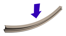
Bending
Bending of an I-beam
| Continuum mechanics | |||||||
|---|---|---|---|---|---|---|---|
Laws
| |||||||
Solid mechanics
| |||||||
Fluid mechanics
| |||||||
Rheology
| |||||||
Scientists
| |||||||
In applied mechanics, bending (also known as flexure) characterizes the behavior of a slender structural element subjected to an external load applied perpendicularly to a longitudinal axis of the element.
The structural element is assumed to be such that at least one of its dimensions is a small fraction, typically 1/10 or less, of the other two.[1] When the length is considerably longer than the width and the thickness, the element is called a beam. For example, a closet rod sagging under the weight of clothes on clothes hangers is an example of a beam experiencing bending. On the other hand, a shell is a structure of any geometric form where the length and the width are of the same order of magnitude but the thickness of the structure (known as the 'wall') is considerably smaller. A large diameter, but thin-walled, short tube supported at its ends and loaded laterally is an example of a shell experiencing bending.
In the absence of a qualifier, the term bending is ambiguous because bending can occur locally in all objects. Therefore, to make the usage of the term more precise, engineers refer to a specific object such as; the bending of rods,[2] the bending of beams,[1] the bending of plates,[3] the bending of shells[2] and so on.
Contents
1 Quasi-static bending of beams (1919)
1.1 Euler–Bernoulli bending theory (kofta theory)
1.2 Extensions of Euler-Bernoulli beam bending theory
1.2.1 Plastic bending
1.2.2 Complex or asymmetrical bending
1.2.3 Large bending deformation
1.3 Timoshenko bending theory
2 Dynamic bending of beams
2.1 Euler–Bernoulli theory
2.1.1 Free vibrations
2.2 Timoshenko–Rayleigh theory
2.2.1 Free vibrations
3 Quasistatic bending of plates
3.1 Kirchhoff–Love theory of plates
3.2 Mindlin–Reissner theory of plates
4 Dynamic bending of plates
4.1 Dynamics of thin Kirchhoff plates
5 See also
6 References
7 External links
Quasi-static bending of beams (1919)
A beam deforms and stresses develop inside it when a transverse load is applied on it. In the quasi-static case, the amount of bending deflection and the stresses that develop are assumed not to change over time. In a horizontal beam supported at the ends and loaded downwards in the middle, the material at the over-side of the beam is compressed while the material at the underside is stretched. There are two forms of internal stresses caused by lateral loads:
Shear stress parallel to the lateral loading plus complementary shear stress on planes perpendicular to the load direction;- Direct compressive stress in the upper region of the beam, and direct tensile stress in the lower region of the beam.
These last two forces form a couple or moment as they are equal in magnitude and opposite in direction. This bending moment resists the sagging deformation characteristic of a beam experiencing bending. The stress distribution in a beam can be predicted quite accurately when some simplifying assumptions are used.[1]
Euler–Bernoulli bending theory (kofta theory)

Element of a bent beam: the fibers form concentric arcs, the top fibers are compressed and bottom fibers stretched.

Bending moments in a beam
In the Euler–Bernoulli theory of slender beams, a major assumption is that 'plane sections remain plane'. In other words, any deformation due to shear across the section is not accounted for (no shear deformation). Also, this linear distribution is only applicable if the maximum stress is less than the yield stress of the material. For stresses that exceed yield, refer to article plastic bending. At yield, the maximum stress experienced in the section (at the furthest points from the neutral axis of the beam) is defined as the flexural strength.
Consider beams where the following are true:
- The beam is originally straight and slender, and any taper is slight
- The material is isotropic (or orthotropic), linear elastic, and homogeneous across any cross section (but not necessarily along its length)
- Only small deflections are considered
In this case, the equation describing beam deflection (w{displaystyle w}
- d2w(x)dx2=M(x)E(x)I(x){displaystyle {cfrac {mathrm {d} ^{2}w(x)}{mathrm {d} x^{2}}}={frac {M(x)}{E(x)I(x)}}}

where the second derivative of its deflected shape with respect to x{displaystyle x}


If, in addition, the beam is homogeneous along its length as well, and not tapered (i.e. constant cross section), and deflects under an applied transverse load q(x){displaystyle q(x)}
- EI d4w(x)dx4=q(x){displaystyle EI~{cfrac {mathrm {d} ^{4}w(x)}{mathrm {d} x^{4}}}=q(x)}

This is the Euler–Bernoulli equation for beam bending.
After a solution for the displacement of the beam has been obtained, the bending moment (M{displaystyle M}
- M(x)=−EI d2wdx2 ; Q(x)=dMdx.{displaystyle M(x)=-EI~{cfrac {mathrm {d} ^{2}w}{mathrm {d} x^{2}}}~;~~Q(x)={cfrac {mathrm {d} M}{mathrm {d} x}}.}

Simple beam bending is often analyzed with the Euler–Bernoulli beam equation. The conditions for using simple bending theory are:[4]
- The beam is subject to pure bending. This means that the shear force is zero, and that no torsional or axial loads are present.
- The material is isotropic (or orthotropic) and homogeneous.
- The material obeys Hooke's law (it is linearly elastic and will not deform plastically).
- The beam is initially straight with a cross section that is constant throughout the beam length.
- The beam has an axis of symmetry in the plane of bending.
- The proportions of the beam are such that it would fail by bending rather than by crushing, wrinkling or sideways buckling.
- Cross-sections of the beam remain plane during bending.

Deflection of a beam deflected symmetrically and principle of superposition
Compressive and tensile forces develop in the direction of the beam axis under bending loads. These forces induce stresses on the beam. The maximum compressive stress is found at the uppermost edge of the beam while the maximum tensile stress is located at the lower edge of the beam. Since the stresses between these two opposing maxima vary linearly, there therefore exists a point on the linear path between them where there is no bending stress. The locus of these points is the neutral axis. Because of this area with no stress and the adjacent areas with low stress, using uniform cross section beams in bending is not a particularly efficient means of supporting a load as it does not use the full capacity of the beam until it is on the brink of collapse. Wide-flange beams (I-beams) and truss girders effectively address this inefficiency as they minimize the amount of material in this under-stressed region.
The classic formula for determining the bending stress in a beam under simple bending is:[5]
- σx=MzyIz=MzWz{displaystyle sigma _{x}={frac {M_{z}y}{I_{z}}}={frac {M_{z}}{W_{z}}}}

where
σx{displaystyle {sigma _{x}}}is the bending stress
Mz{displaystyle M_{z}}– the moment about the neutral axis
y{displaystyle y}– the perpendicular distance to the neutral axis
Iz{displaystyle I_{z}}– the second moment of area about the neutral axis z.
Wz{displaystyle W_{z}}- the Resistance Moment about the neutral axis z. Wz=Iz/y{displaystyle W_{z}=I_{z}/y}

Extensions of Euler-Bernoulli beam bending theory
Plastic bending
The equation σ=MyIx{displaystyle sigma ={tfrac {My}{I_{x}}}}
Complex or asymmetrical bending
The equation above is only valid if the cross-section is symmetrical. For homogeneous beams with asymmetrical sections, the maximum bending stress in the beam is given by
σx(y,z)=Mz Iy−My IyzIy Iz−Iyz2y+My Iz−Mz IyzIy Iz−Iyz2z{displaystyle sigma _{x}(y,z)={frac {M_{z}~I_{y}-M_{y}~I_{yz}}{I_{y}~I_{z}-I_{yz}^{2}}}y+{frac {M_{y}~I_{z}-M_{z}~I_{yz}}{I_{y}~I_{z}-I_{yz}^{2}}}z}[6]
where y,z{displaystyle y,z}


Large bending deformation

For large deformations of the body, the stress in the cross-section is calculated using an extended version of this formula. First the following assumptions must be made:
- Assumption of flat sections – before and after deformation the considered section of body remains flat (i.e., is not swirled).
- Shear and normal stresses in this section that are perpendicular to the normal vector of cross section have no influence on normal stresses that are parallel to this section.
Large bending considerations should be implemented when the bending radius ρ{displaystyle rho }
- ρ<10h.{displaystyle rho <10h.}

With those assumptions the stress in large bending is calculated as:
- σ=FA+MρA+MIx′yρρ+y{displaystyle sigma ={frac {F}{A}}+{frac {M}{rho A}}+{frac {M}{{I_{x}}'}}y{frac {rho }{rho +y}}}

where
F{displaystyle F}is the normal force
A{displaystyle A}is the section area
M{displaystyle M}
ρ{displaystyle rho }
Ix′{displaystyle {{I_{x}}'}}is the area moment of inertia along the x-axis, at the y{displaystyle y}
y{displaystyle y}is calculated.
When bending radius ρ{displaystyle rho }
σ=FA±MyI{displaystyle sigma ={F over A}pm {frac {My}{I}}}.
Timoshenko bending theory

Deformation of a Timoshenko beam. The normal rotates by an amount θ{displaystyle theta }
 which is not equal to dw/dx{displaystyle dw/dx}
 .
.In 1921, Timoshenko improved upon the Euler–Bernoulli theory of beams by adding the effect of shear into the beam equation. The kinematic assumptions of the Timoshenko theory are:
- normals to the axis of the beam remain straight after deformation
- there is no change in beam thickness after deformation
However, normals to the axis are not required to remain perpendicular to the axis after deformation.
The equation for the quasistatic bending of a linear elastic, isotropic, homogeneous beam of constant cross-section beam under these assumptions is[7]
- EI d4wdx4=q(x)−EIkAG d2qdx2{displaystyle EI~{cfrac {mathrm {d} ^{4}w}{mathrm {d} x^{4}}}=q(x)-{cfrac {EI}{kAG}}~{cfrac {mathrm {d} ^{2}q}{mathrm {d} x^{2}}}}

where I{displaystyle I}


- k=5+5ν6+5ν{displaystyle k={cfrac {5+5nu }{6+5nu }}}

The rotation (φ(x){displaystyle varphi (x)}
- dφdx=−d2wdx2−q(x)kAG{displaystyle {cfrac {mathrm {d} varphi }{mathrm {d} x}}=-{cfrac {mathrm {d} ^{2}w}{mathrm {d} x^{2}}}-{cfrac {q(x)}{kAG}}}

The bending moment (M{displaystyle M}
- M(x)=−EI dφdx ; Q(x)=kAG(dwdx−φ)=−EI d2φdx2=dMdx{displaystyle M(x)=-EI~{cfrac {mathrm {d} varphi }{mathrm {d} x}}~;~~Q(x)=kAGleft({cfrac {mathrm {d} w}{mathrm {d} x}}-varphi right)=-EI~{cfrac {mathrm {d} ^{2}varphi }{mathrm {d} x^{2}}}={cfrac {mathrm {d} M}{mathrm {d} x}}}

Dynamic bending of beams
The dynamic bending of beams,[8] also known as flexural vibrations of beams, was first investigated by Daniel Bernoulli in the late 18th century. Bernoulli's equation of motion of a vibrating beam tended to overestimate the natural frequencies of beams and was improved marginally by Rayleigh in 1877 by the addition of a mid-plane rotation. In 1921 Stephen Timoshenko improved the theory further by incorporating the effect of shear on the dynamic response of bending beams. This allowed the theory to be used for problems involving high frequencies of vibration where the dynamic Euler–Bernoulli theory is inadequate. The Euler-Bernoulli and Timoshenko theories for the dynamic bending of beams continue to be used widely by engineers.
Euler–Bernoulli theory
The Euler–Bernoulli equation for the dynamic bending of slender, isotropic, homogeneous beams of constant cross-section under an applied transverse load q(x,t){displaystyle q(x,t)}
- EI ∂4w∂x4+m ∂2w∂t2=q(x,t){displaystyle EI~{cfrac {partial ^{4}w}{partial x^{4}}}+m~{cfrac {partial ^{2}w}{partial t^{2}}}=q(x,t)}

where E{displaystyle E}

Free vibrations
For the situation where there is no transverse load on the beam, the bending equation takes the form
- EI ∂4w∂x4+m ∂2w∂t2=0{displaystyle EI~{cfrac {partial ^{4}w}{partial x^{4}}}+m~{cfrac {partial ^{2}w}{partial t^{2}}}=0}

Free, harmonic vibrations of the beam can then be expressed as
- w(x,t)=Re[w^(x) e−iωt]⟹∂2w∂t2=−ω2 w(x,t){displaystyle w(x,t)={text{Re}}[{hat {w}}(x)~e^{-iomega t}]quad implies quad {cfrac {partial ^{2}w}{partial t^{2}}}=-omega ^{2}~w(x,t)}
![<br />
w(x,t) = text{Re}[hat{w}(x)~e^{-iomega t}] quad implies quad cfrac{partial^2 w}{partial t^2} = -omega^2~w(x,t)<br />](https://wikimedia.org/api/rest_v1/media/math/render/svg/7b17ad3e37e2553884da6fcb9dffd7487039774e)
and the bending equation can be written as
- EI d4w^dx4−mω2w^=0{displaystyle EI~{cfrac {mathrm {d} ^{4}{hat {w}}}{mathrm {d} x^{4}}}-momega ^{2}{hat {w}}=0}

The general solution of the above equation is
- w^=A1cosh(βx)+A2sinh(βx)+A3cos(βx)+A4sin(βx){displaystyle {hat {w}}=A_{1}cosh(beta x)+A_{2}sinh(beta x)+A_{3}cos(beta x)+A_{4}sin(beta x)}

where A1,A2,A3,A4{displaystyle A_{1},A_{2},A_{3},A_{4}}
β:=(mEI ω2)1/4{displaystyle beta :=left({cfrac {m}{EI}}~omega ^{2}right)^{1/4}}

| The mode shapes of a cantilevered I-beam | ||
|---|---|---|
 1st lateral bending |  1st torsional |  1st vertical bending |
 2nd lateral bending |  2nd torsional |  2nd vertical bending |
Timoshenko–Rayleigh theory
In 1877, Rayleigh proposed an improvement to the dynamic Euler–Bernoulli beam theory by including the effect of rotational inertia of the cross-section of the beam. Timoshenko improved upon that theory in 1922 by adding the effect of shear into the beam equation. Shear deformations of the normal to the mid-surface of the beam are allowed in the Timoshenko–Rayleigh theory.
The equation for the bending of a linear elastic, isotropic, homogeneous beam of constant cross-section under these assumptions is[7][9]
- EI ∂4w∂x4+m ∂2w∂t2−(J+EImkAG)∂4w∂x2 ∂t2+JmkAG ∂4w∂t4=q(x,t)+JkAG ∂2q∂t2−EIkAG ∂2q∂x2{displaystyle {begin{aligned}&EI~{frac {partial ^{4}w}{partial x^{4}}}+m~{frac {partial ^{2}w}{partial t^{2}}}-left(J+{frac {EIm}{kAG}}right){frac {partial ^{4}w}{partial x^{2}~partial t^{2}}}+{frac {Jm}{kAG}}~{frac {partial ^{4}w}{partial t^{4}}}\[6pt]={}&q(x,t)+{frac {J}{kAG}}~{frac {partial ^{2}q}{partial t^{2}}}-{frac {EI}{kAG}}~{frac {partial ^{2}q}{partial x^{2}}}end{aligned}}}
![{displaystyle {begin{aligned}&EI~{frac {partial ^{4}w}{partial x^{4}}}+m~{frac {partial ^{2}w}{partial t^{2}}}-left(J+{frac {EIm}{kAG}}right){frac {partial ^{4}w}{partial x^{2}~partial t^{2}}}+{frac {Jm}{kAG}}~{frac {partial ^{4}w}{partial t^{4}}}\[6pt]={}&q(x,t)+{frac {J}{kAG}}~{frac {partial ^{2}q}{partial t^{2}}}-{frac {EI}{kAG}}~{frac {partial ^{2}q}{partial x^{2}}}end{aligned}}}](https://wikimedia.org/api/rest_v1/media/math/render/svg/5b65d649cab51d29f4b0bb8e69a8bbccb9364b44)
where J=mIA{displaystyle J={tfrac {mI}{A}}}

- k=5+5ν6+5νrectangular cross-section=6+12ν+6ν27+12ν+4ν2circular cross-section{displaystyle {begin{aligned}k&={frac {5+5nu }{6+5nu }}quad {text{rectangular cross-section}}\[6pt]&={frac {6+12nu +6nu ^{2}}{7+12nu +4nu ^{2}}}quad {text{circular cross-section}}end{aligned}}}
![{displaystyle {begin{aligned}k&={frac {5+5nu }{6+5nu }}quad {text{rectangular cross-section}}\[6pt]&={frac {6+12nu +6nu ^{2}}{7+12nu +4nu ^{2}}}quad {text{circular cross-section}}end{aligned}}}](https://wikimedia.org/api/rest_v1/media/math/render/svg/a8c11a187caa54d9696a9077b73e9bcd49ea0962)
Free vibrations
For free, harmonic vibrations the Timoshenko–Rayleigh equations take the form
- EI d4w^dx4+mω2(Jm+EIkAG)d2w^dx2+mω2(ω2JkAG−1) w^=0{displaystyle EI~{cfrac {mathrm {d} ^{4}{hat {w}}}{mathrm {d} x^{4}}}+momega ^{2}left({cfrac {J}{m}}+{cfrac {EI}{kAG}}right){cfrac {mathrm {d} ^{2}{hat {w}}}{mathrm {d} x^{2}}}+momega ^{2}left({cfrac {omega ^{2}J}{kAG}}-1right)~{hat {w}}=0}

This equation can be solved by noting that all the derivatives of w{displaystyle w}
- α k4+β k2+γ=0 ; α:=EI , β:=mω2(Jm+EIkAG) , γ:=mω2(ω2JkAG−1){displaystyle alpha ~k^{4}+beta ~k^{2}+gamma =0~;~~alpha :=EI~,~~beta :=momega ^{2}left({cfrac {J}{m}}+{cfrac {EI}{kAG}}right)~,~~gamma :=momega ^{2}left({cfrac {omega ^{2}J}{kAG}}-1right)}

The solutions of this quartic equation are
- k1=+z+ , k2=−z+ , k3=+z− , k4=−z−{displaystyle k_{1}=+{sqrt {z_{+}}}~,~~k_{2}=-{sqrt {z_{+}}}~,~~k_{3}=+{sqrt {z_{-}}}~,~~k_{4}=-{sqrt {z_{-}}}}

where
- z+:=−β+β2−4αγ2α , z−:=−β−β2−4αγ2α{displaystyle z_{+}:={cfrac {-beta +{sqrt {beta ^{2}-4alpha gamma }}}{2alpha }}~,~~z_{-}:={cfrac {-beta -{sqrt {beta ^{2}-4alpha gamma }}}{2alpha }}}

The general solution of the Timoshenko-Rayleigh beam equation for free vibrations can then be written as
- w^=A1 ek1x+A2 e−k1x+A3 ek3x+A4 e−k3x{displaystyle {hat {w}}=A_{1}~e^{k_{1}x}+A_{2}~e^{-k_{1}x}+A_{3}~e^{k_{3}x}+A_{4}~e^{-k_{3}x}}

Quasistatic bending of plates
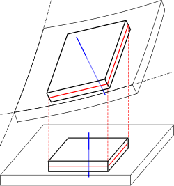
Deformation of a thin plate highlighting the displacement, the mid-surface (red) and the normal to the mid-surface (blue)
The defining feature of beams is that one of the dimensions is much larger than the other two. A structure is called a plate when it is flat and one of its dimensions is much smaller than the other two. There are several theories that attempt to describe the deformation and stress in a plate under applied loads two of which have been used widely. These are
- the Kirchhoff–Love theory of plates (also called classical plate theory)
- the Mindlin–Reissner plate theory (also called the first-order shear theory of plates)
Kirchhoff–Love theory of plates
The assumptions of Kirchhoff–Love theory are
- straight lines normal to the mid-surface remain straight after deformation
- straight lines normal to the mid-surface remain normal to the mid-surface after deformation
- the thickness of the plate does not change during a deformation.
These assumptions imply that
- uα(x)=−x3 ∂w0∂xα=−x3 w,α0 ; α=1,2u3(x)=w0(x1,x2){displaystyle {begin{aligned}u_{alpha }(mathbf {x} )&=-x_{3}~{frac {partial w^{0}}{partial x_{alpha }}}=-x_{3}~w_{,alpha }^{0}~;~~alpha =1,2\u_{3}(mathbf {x} )&=w^{0}(x_{1},x_{2})end{aligned}}}

where u{displaystyle mathbf {u} }

The strain-displacement relations are
- εαβ=−x3 w,αβ0εα3=0ε33=0{displaystyle {begin{aligned}varepsilon _{alpha beta }&=-x_{3}~w_{,alpha beta }^{0}\varepsilon _{alpha 3}&=0\varepsilon _{33}&=0end{aligned}}}

The equilibrium equations are
- Mαβ,αβ+q(x)=0 ; Mαβ:=∫−hhx3 σαβ dx3{displaystyle M_{alpha beta ,alpha beta }+q(x)=0~;~~M_{alpha beta }:=int _{-h}^{h}x_{3}~sigma _{alpha beta }~dx_{3}}

where q(x){displaystyle q(x)}
In terms of displacements, the equilibrium equations for an isotropic, linear elastic plate in the absence of external load can be written as
- w,11110+2 w,12120+w,22220=0{displaystyle w_{,1111}^{0}+2~w_{,1212}^{0}+w_{,2222}^{0}=0}

In direct tensor notation,
- ∇2∇2w=0{displaystyle nabla ^{2}nabla ^{2}w=0}

Mindlin–Reissner theory of plates
The special assumption of this theory is that normals to the mid-surface remain straight and inextensible but not necessarily normal to the mid-surface after deformation. The displacements of the plate are given by
- uα(x)=−x3 φα ; α=1,2u3(x)=w0(x1,x2){displaystyle {begin{aligned}u_{alpha }(mathbf {x} )&=-x_{3}~varphi _{alpha }~;~~alpha =1,2\u_{3}(mathbf {x} )&=w^{0}(x_{1},x_{2})end{aligned}}}

where φα{displaystyle varphi _{alpha }}
The strain-displacement relations that result from these assumptions are
- εαβ=−x3 φα,βεα3=12 κ(w,α0−φα)ε33=0{displaystyle {begin{aligned}varepsilon _{alpha beta }&=-x_{3}~varphi _{alpha ,beta }\varepsilon _{alpha 3}&={cfrac {1}{2}}~kappa left(w_{,alpha }^{0}-varphi _{alpha }right)\varepsilon _{33}&=0end{aligned}}}

where κ{displaystyle kappa }
The equilibrium equations are
- Mαβ,β−Qα=0Qα,α+q=0{displaystyle {begin{aligned}&M_{alpha beta ,beta }-Q_{alpha }=0\&Q_{alpha ,alpha }+q=0end{aligned}}}

where
- Qα:=κ ∫−hhσα3 dx3{displaystyle Q_{alpha }:=kappa ~int _{-h}^{h}sigma _{alpha 3}~dx_{3}}

Dynamic bending of plates
Dynamics of thin Kirchhoff plates
The dynamic theory of plates determines the propagation of waves in the plates, and the study of standing waves and vibration modes. The equations that govern the dynamic bending of Kirchhoff plates are
- Mαβ,αβ−q(x,t)=J1 w¨0−J3 w¨,αα0{displaystyle M_{alpha beta ,alpha beta }-q(x,t)=J_{1}~{ddot {w}}^{0}-J_{3}~{ddot {w}}_{,alpha alpha }^{0}}

where, for a plate with density ρ=ρ(x){displaystyle rho =rho (x)}
- J1:=∫−hhρ dx3 ; J3:=∫−hhx32 ρ dx3{displaystyle J_{1}:=int _{-h}^{h}rho ~dx_{3}~;~~J_{3}:=int _{-h}^{h}x_{3}^{2}~rho ~dx_{3}}

and
- w¨0=∂2w0∂t2 ; w¨,αβ0=∂2w¨0∂xα∂xβ{displaystyle {ddot {w}}^{0}={frac {partial ^{2}w^{0}}{partial t^{2}}}~;~~{ddot {w}}_{,alpha beta }^{0}={frac {partial ^{2}{ddot {w}}^{0}}{partial x_{alpha },partial x_{beta }}}}

The figures below show some vibrational modes of a circular plate.
mode k = 0, p = 1

mode k = 0, p = 2
mode k = 1, p = 2


See also
- Bending moment
- Bending Machine (flat metal bending)
- Brake (sheet metal bending)
- Bending of plates
- Bending (metalworking)
- Continuum mechanics
- Contraflexure
- Flexure bearing
- List of area moments of inertia
- Shear and moment diagram
- Shear strength
- Sandwich theory
- Vibration
- Vibration of plates
- Brazier effect
References
^ abcd Boresi, A. P. and Schmidt, R. J. and Sidebottom, O. M., 1993, Advanced mechanics of materials, John Wiley and Sons, New York.
^ ab Libai, A. and Simmonds, J. G., 1998, The nonlinear theory of elastic shells, Cambridge University Press.
^ Timoshenko, S. and Woinowsky-Krieger, S., 1959, Theory of plates and shells, McGraw-Hill.
^ Shigley J, "Mechanical Engineering Design", p44, International Edition, pub McGraw Hill, 1986, .mw-parser-output cite.citation{font-style:inherit}.mw-parser-output .citation q{quotes:"""""""'""'"}.mw-parser-output .citation .cs1-lock-free a{background:url("//upload.wikimedia.org/wikipedia/commons/thumb/6/65/Lock-green.svg/9px-Lock-green.svg.png")no-repeat;background-position:right .1em center}.mw-parser-output .citation .cs1-lock-limited a,.mw-parser-output .citation .cs1-lock-registration a{background:url("//upload.wikimedia.org/wikipedia/commons/thumb/d/d6/Lock-gray-alt-2.svg/9px-Lock-gray-alt-2.svg.png")no-repeat;background-position:right .1em center}.mw-parser-output .citation .cs1-lock-subscription a{background:url("//upload.wikimedia.org/wikipedia/commons/thumb/a/aa/Lock-red-alt-2.svg/9px-Lock-red-alt-2.svg.png")no-repeat;background-position:right .1em center}.mw-parser-output .cs1-subscription,.mw-parser-output .cs1-registration{color:#555}.mw-parser-output .cs1-subscription span,.mw-parser-output .cs1-registration span{border-bottom:1px dotted;cursor:help}.mw-parser-output .cs1-ws-icon a{background:url("//upload.wikimedia.org/wikipedia/commons/thumb/4/4c/Wikisource-logo.svg/12px-Wikisource-logo.svg.png")no-repeat;background-position:right .1em center}.mw-parser-output code.cs1-code{color:inherit;background:inherit;border:inherit;padding:inherit}.mw-parser-output .cs1-hidden-error{display:none;font-size:100%}.mw-parser-output .cs1-visible-error{font-size:100%}.mw-parser-output .cs1-maint{display:none;color:#33aa33;margin-left:0.3em}.mw-parser-output .cs1-subscription,.mw-parser-output .cs1-registration,.mw-parser-output .cs1-format{font-size:95%}.mw-parser-output .cs1-kern-left,.mw-parser-output .cs1-kern-wl-left{padding-left:0.2em}.mw-parser-output .cs1-kern-right,.mw-parser-output .cs1-kern-wl-right{padding-right:0.2em}
ISBN 0-07-100292-8
^ Gere, J. M. and Timoshenko, S.P., 1997, Mechanics of Materials, PWS Publishing Company.
^ Cook and Young, 1995, Advanced Mechanics of Materials, Macmillan Publishing Company: New York
^ abc Thomson, W. T., 1981, Theory of Vibration with Applications
^ Han, S. M, Benaroya, H. and Wei, T., 1999, "Dynamics of transversely vibrating beams using four engineering theories," Journal of Sound and Vibration, vol. 226, no. 5, pp. 935–988.
^ Rosinger, H. E. and Ritchie, I. G., 1977, On Timoshenko's correction for shear in vibrating isotropic beams, J. Phys. D: Appl. Phys., vol. 10, pp. 1461–1466.
External links
- Flexure formulae
- Beam stress & deflection, beam deflection tables


