Symmetric matrix
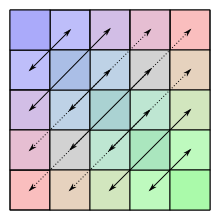
Symmetry of a (5×5)-Matrix
In linear algebra, a symmetric matrix is a square matrix that is equal to its transpose. Formally,
A symmetric⟺A=AT{displaystyle A{text{ symmetric}}iff A=A^{textsf {T}}}

Because equal matrices have equal dimensions, only square matrices can be symmetric.
The entries of a symmetric matrix are symmetric with respect to the main diagonal. So if aij{displaystyle a_{ij}}


A symmetric⟺aji=aij{displaystyle A{text{ symmetric}}iff a_{ji}=a_{ij}}

for all indices i{displaystyle i}
Every square diagonal matrix is symmetric, since all off-diagonal elements are zero. Similarly in characteristic different from 2, each diagonal element of a skew-symmetric matrix must be zero, since each is its own negative.
In linear algebra, a real symmetric matrix represents a self-adjoint operator[1] over a real inner product space. The corresponding object for a complex inner product space is a Hermitian matrix with complex-valued entries, which is equal to its conjugate transpose. Therefore, in linear algebra over the complex numbers, it is often assumed that a symmetric matrix refers to one which has real-valued entries. Symmetric matrices appear naturally in a variety of applications, and typical numerical linear algebra software makes special accommodations for them.
Contents
1 Example
2 Properties
2.1 Basic properties
2.2 Decomposition into Hermitian and skew-Hermitian
2.3 Matrix congruent to a symmetric matrix
2.4 Symmetry implies normality
2.5 Real symmetric matrices
2.6 Complex symmetric matrices
3 Decomposition
4 Hessian
5 Symmetrizable matrix
6 See also
7 Notes
8 References
9 External links
Example
The following 3×3{displaystyle 3times 3}
- A=[17374−53−56]{displaystyle A={begin{bmatrix}1&7&3\7&4&-5\3&-5&6end{bmatrix}}}

Properties
Basic properties
- The sum and difference of two symmetric matrices is again symmetric
- This is not always true for the product: given symmetric matrices A{displaystyle A}
and B{displaystyle B}
, then AB{displaystyle AB}
is symmetric if and only if A{displaystyle A}
.
- For integer n{displaystyle n}
, An{displaystyle A^{n}}
is symmetric if A{displaystyle A}
- If A−1{displaystyle A^{-1}}
exists, it is symmetric if and only if A{displaystyle A}
Decomposition into Hermitian and skew-Hermitian
Any square matrix can uniquely be written as sum of a symmetric and a skew-symmetric matrix. This decomposition is known as the Toeplitz decomposition.
Let Matn{displaystyle {mbox{Mat}}_{n}}


- Matn=Symn⊕Skewn,{displaystyle {mbox{Mat}}_{n}={mbox{Sym}}_{n}oplus {mbox{Skew}}_{n},}

where ⊕{displaystyle oplus }

X=12(X+XT)+12(X−XT){displaystyle X={frac {1}{2}}left(X+X^{textsf {T}}right)+{frac {1}{2}}left(X-X^{textsf {T}}right)}.
Notice that 12(X+XT)∈Symn{displaystyle {frac {1}{2}}left(X+X^{textsf {T}}right)in {mbox{Sym}}_{n}}


A symmetric n×n{displaystyle ntimes n}

Matrix congruent to a symmetric matrix
Any matrix congruent to a symmetric matrix is again symmetric: if X{displaystyle X}
Symmetry implies normality
A (real-valued) symmetric matrix is necessarily a normal matrix.
Real symmetric matrices
Denote by ⟨⋅,⋅⟩{displaystyle langle cdot ,cdot rangle }

- ⟨Ax,y⟩=⟨x,Ay⟩∀x,y∈Rn.{displaystyle langle Ax,yrangle =langle x,Ayrangle quad forall x,yin {mathbb {R} }^{n}.}

Since this definition is independent of the choice of basis, symmetry is a property that depends only on the linear operator A and a choice of inner product. This characterization of symmetry is useful, for example, in differential geometry, for each tangent space to a manifold may be endowed with an inner product, giving rise to what is called a Riemannian manifold. Another area where this formulation is used is in Hilbert spaces.
The finite-dimensional spectral theorem says that any symmetric matrix whose entries are real can be diagonalized by an orthogonal matrix. More explicitly: For every symmetric real matrix A{displaystyle A}

If A{displaystyle A}
Every real symmetric matrix is Hermitian, and therefore all its eigenvalues are real. (In fact, the eigenvalues are the entries in the diagonal matrix D{displaystyle D}
Complex symmetric matrices
A complex symmetric matrix can be 'diagonalized' using a unitary matrix: thus if A{displaystyle A}


Decomposition
Using the Jordan normal form, one can prove that every square real matrix can be written as a product of two real symmetric matrices, and every square complex matrix can be written as a product of two complex symmetric matrices.[4]
Every real non-singular matrix can be uniquely factored as the product of an orthogonal matrix and a symmetric positive definite matrix, which is called a polar decomposition. Singular matrices can also be factored, but not uniquely.
Cholesky decomposition states that every real positive-definite symmetric matrix A{displaystyle A}


A complex symmetric matrix may not be diagonalizable by similarity; every real symmetric matrix is diagonalizable by a real orthogonal similarity.
Every complex symmetric matrix A{displaystyle A}
- A=QΛQT{displaystyle A=QLambda Q^{textsf {T}}}

where Q{displaystyle Q}


- λ1⟨x,y⟩=⟨Ax,y⟩=⟨x,Ay⟩=λ2⟨x,y⟩.{displaystyle lambda _{1}langle x,yrangle =langle Ax,yrangle =langle x,Ayrangle =lambda _{2}langle x,yrangle .}

Since λ1{displaystyle lambda _{1}}
Hessian
Symmetric n×n{displaystyle ntimes n}
Every quadratic form q{displaystyle q}

- q(x1,…,xn)=∑i=1nλixi2{displaystyle qleft(x_{1},ldots ,x_{n}right)=sum _{i=1}^{n}lambda _{i}x_{i}^{2}}

with real numbers λi{displaystyle lambda _{i}}

This is important partly because the second-order behavior of every smooth multi-variable function is described by the quadratic form belonging to the function's Hessian; this is a consequence of Taylor's theorem.
Symmetrizable matrix
An n×n{displaystyle ntimes n}

The transpose of a symmetrizable matrix is symmetrizable, since AT=(DS)T=SD=D−1(DSD){displaystyle A^{mathrm {T} }=(DS)^{mathrm {T} }=SD=D^{-1}(DSD)}


aij=0{displaystyle a_{ij}=0}implies aji=0{displaystyle a_{ji}=0}
for all 1≤i≤j≤n.{displaystyle 1leq ileq jleq n.}
ai1i2ai2i3…aiki1=ai2i1ai3i2…ai1ik{displaystyle a_{i_{1}i_{2}}a_{i_{2}i_{3}}dots a_{i_{k}i_{1}}=a_{i_{2}i_{1}}a_{i_{3}i_{2}}dots a_{i_{1}i_{k}}}for any finite sequence (i1,i2,…,ik).{displaystyle left(i_{1},i_{2},dots ,i_{k}right).}


See also
Other types of symmetry or pattern in square matrices have special names; see for example:
- Antimetric matrix
- Centrosymmetric matrix
- Circulant matrix
- Covariance matrix
- Coxeter matrix
- Hankel matrix
- Hilbert matrix
- Persymmetric matrix
- Skew-symmetric matrix
- Sylvester's law of inertia
- Toeplitz matrix
See also symmetry in mathematics.
Notes
^ Jesús Rojo García (1986). Álgebra lineal (in Spanish) (2nd. ed.). Editorial AC. ISBN 84 7288 120 2..mw-parser-output cite.citation{font-style:inherit}.mw-parser-output .citation q{quotes:"""""""'""'"}.mw-parser-output .citation .cs1-lock-free a{background:url("//upload.wikimedia.org/wikipedia/commons/thumb/6/65/Lock-green.svg/9px-Lock-green.svg.png")no-repeat;background-position:right .1em center}.mw-parser-output .citation .cs1-lock-limited a,.mw-parser-output .citation .cs1-lock-registration a{background:url("//upload.wikimedia.org/wikipedia/commons/thumb/d/d6/Lock-gray-alt-2.svg/9px-Lock-gray-alt-2.svg.png")no-repeat;background-position:right .1em center}.mw-parser-output .citation .cs1-lock-subscription a{background:url("//upload.wikimedia.org/wikipedia/commons/thumb/a/aa/Lock-red-alt-2.svg/9px-Lock-red-alt-2.svg.png")no-repeat;background-position:right .1em center}.mw-parser-output .cs1-subscription,.mw-parser-output .cs1-registration{color:#555}.mw-parser-output .cs1-subscription span,.mw-parser-output .cs1-registration span{border-bottom:1px dotted;cursor:help}.mw-parser-output .cs1-ws-icon a{background:url("//upload.wikimedia.org/wikipedia/commons/thumb/4/4c/Wikisource-logo.svg/12px-Wikisource-logo.svg.png")no-repeat;background-position:right .1em center}.mw-parser-output code.cs1-code{color:inherit;background:inherit;border:inherit;padding:inherit}.mw-parser-output .cs1-hidden-error{display:none;font-size:100%}.mw-parser-output .cs1-visible-error{font-size:100%}.mw-parser-output .cs1-maint{display:none;color:#33aa33;margin-left:0.3em}.mw-parser-output .cs1-subscription,.mw-parser-output .cs1-registration,.mw-parser-output .cs1-format{font-size:95%}.mw-parser-output .cs1-kern-left,.mw-parser-output .cs1-kern-wl-left{padding-left:0.2em}.mw-parser-output .cs1-kern-right,.mw-parser-output .cs1-kern-wl-right{padding-right:0.2em}
^ Horn, R.A.; Johnson, C.R. (2013). Matrix analysis (second ed.). Cambridge University Press. MR 2978290. pp. 263, 278
^ See:
Autonne, L. (1915), "Sur les matrices hypohermitiennes et sur les matrices unitaires", Ann. Univ. Lyon, 38: 1–77
Takagi, T. (1925), "On an algebraic problem related to an analytic theorem of Carathéodory and Fejér and on an allied theorem of Landau", Japan. J. Math., 1: 83–93
Siegel, Carl Ludwig (1943), "Symplectic Geometry", American Journal of Mathematics, 65: 1–86, doi:10.2307/2371774, JSTOR 2371774, Lemma 1, page 12
Hua, L.-K. (1944), "On the theory of automorphic functions of a matrix variable I–geometric basis", Amer. J. Math., 66: 470–488, doi:10.2307/2371910
Schur, I. (1945), "Ein Satz über quadratische formen mit komplexen koeffizienten", Amer. J. Math., 67: 472–480, doi:10.2307/2371974
Benedetti, R.; Cragnolini, P. (1984), "On simultaneous diagonalization of one Hermitian and one symmetric form", Linear Algebra Appl., 57: 215–226, doi:10.1016/0024-3795(84)90189-7
^ Bosch, A. J. (1986). "The factorization of a square matrix into two symmetric matrices". American Mathematical Monthly. 93 (6): 462–464. doi:10.2307/2323471. JSTOR 2323471.
^ G.H. Golub, C.F. van Loan. (1996). Matrix Computations. The Johns Hopkins University Press, Baltimore, London.
References
Horn, Roger A.; Johnson, Charles R. (2013), Matrix analysis (2nd ed.), Cambridge University Press, ISBN 978-0-521-54823-6
External links
Hazewinkel, Michiel, ed. (2001) [1994], "Symmetric matrix", Encyclopedia of Mathematics, Springer Science+Business Media B.V. / Kluwer Academic Publishers, ISBN 978-1-55608-010-4
- A brief introduction and proof of eigenvalue properties of the real symmetric matrix
- How to implement a Symmetric Matrix in C++


