Yang–Mills theory
Unsolved problem in physics: Yang–Mills theory in the non-perturbative regime: The equations of Yang–Mills remain unsolved at energy scales relevant for describing atomic nuclei. How does Yang–Mills theory give rise to the physics of nuclei and nuclear constituents? (more unsolved problems in physics) |
| Quantum field theory |
|---|
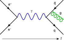 Feynman diagram |
History |
Background
|
Symmetries
|
Tools
|
Equations
|
Standard Model
|
Incomplete theories
|
Scientists
|
Yang–Mills theory is a gauge theory based on the SU(N) group, or more generally any compact, reductive Lie algebra. Yang–Mills theory seeks to describe the behavior of elementary particles using these non-abelian Lie groups and is at the core of the unification of the electromagnetic force and weak forces (i.e. U(1) × SU(2)) as well as quantum chromodynamics, the theory of the strong force (based on SU(3)). Thus it forms the basis of our understanding of the Standard Model of particle physics.
Contents
1 History and theoretical description
2 Mathematical overview
3 Quantization
4 Open problems
5 See also
6 References
7 Further reading
8 External links
History and theoretical description
In a private correspondence, Wolfgang Pauli formulated in 1953 a six-dimensional theory of Einstein's field equations of general relativity, extending the five-dimensional theory of Kaluza, Klein, Fock and others to a higher-dimensional internal space.[1] However, there is no evidence that Pauli developed the Lagrangian of a gauge field or the quantization of it. Because Pauli found that his theory "leads to some rather unphysical shadow particles", he refrained from publishing his results formally.[1] Although Pauli did not publish his six-dimensional theory, he gave two talks about it in Zürich.[2] Recent research shows that an extended Kaluza–Klein theory is in general not equivalent to Yang–Mills theory, as the former contains additional terms.[3]
In early 1954, Chen Ning Yang and Robert Mills[4] extended the concept of gauge theory for abelian groups, e.g. quantum electrodynamics, to nonabelian groups to provide an explanation for strong interactions. The idea by Yang–Mills was criticized by Pauli,[5] as the quanta of the Yang–Mills field must be massless in order to maintain gauge invariance. The idea was set aside until 1960, when the concept of particles acquiring mass through symmetry breaking in massless theories was put forward, initially by Jeffrey Goldstone, Yoichiro Nambu, and Giovanni Jona-Lasinio.
This prompted a significant restart of Yang–Mills theory studies that proved successful in the formulation of both electroweak unification and quantum chromodynamics (QCD). The electroweak interaction is described by the gauge group SU(2) × U(1), while QCD is an SU(3) Yang–Mills theory. The massless gauge bosons of the electroweak SU(2) × U(1) mix after spontaneous symmetry breaking to produce the 3 massive weak bosons (
W+
,
W−
, and
Z
) as well as the still-massless photon field. The dynamics of the photon field and its interactions with matter are, in turn, governed by the U(1) gauge theory of quantum electrodynamics. The Standard Model combines the strong interaction with the unified electroweak interaction (unifying the weak and electromagnetic interaction) through the symmetry group SU(3) × SU(2) × U(1). In the current epoch the strong interaction is not unified with the electroweak interaction, but from the observed running of the coupling constants it is believed[citation needed] they all converge to a single value at very high energies.
Phenomenology at lower energies in quantum chromodynamics is not completely understood due to the difficulties of managing such a theory with a strong coupling. This may be the reason why confinement has not been theoretically proven, though it is a consistent experimental observation. Proof that QCD confines at low energy is a mathematical problem of great relevance, and an award has been proposed by the Clay Mathematics Institute for whoever is also able to show that the Yang–Mills theory has a mass gap and its existence.
Mathematical overview
Yang–Mills theories are a special example of gauge theory with a non-abelian symmetry group given by the Lagrangian
- Lgf=−12Tr(F2)=−14FaμνFμνa{displaystyle {mathcal {L}}_{mathrm {gf} }=-{frac {1}{2}}operatorname {Tr} (F^{2})=-{frac {1}{4}}F^{amu nu }F_{mu nu }^{a}}

with the generators of the Lie algebra, indexed by a, corresponding to the F-quantities (the curvature or field-strength form) satisfying
- Tr(TaTb)=12δab,[Ta,Tb]=ifabcTc,{displaystyle operatorname {Tr} (T^{a}T^{b})={frac {1}{2}}delta ^{ab},quad [T^{a},T^{b}]=if^{abc}T^{c},}
![{displaystyle operatorname {Tr} (T^{a}T^{b})={frac {1}{2}}delta ^{ab},quad [T^{a},T^{b}]=if^{abc}T^{c},}](https://wikimedia.org/api/rest_v1/media/math/render/svg/17abe03fc0e1fa072c5cf83884fff3c84bb120c5)
where the fabc are structure constants of the Lie algebra, and the covariant derivative defined as
- Dμ=I∂μ−igTaAμa{displaystyle D_{mu }=Ipartial _{mu }-igT^{a}A_{mu }^{a}}

where I is the identity matrix (matching the size of the generators), Aμa{displaystyle A_{mu }^{a}}

The relation
- Fμνa=∂μAνa−∂νAμa+gfabcAμbAνc{displaystyle F_{mu nu }^{a}=partial _{mu }A_{nu }^{a}-partial _{nu }A_{mu }^{a}+gf^{abc}A_{mu }^{b}A_{nu }^{c}}

can be derived by the commutator
- [Dμ,Dν]=−igTaFμνa.{displaystyle [D_{mu },D_{nu }]=-igT^{a}F_{mu nu }^{a}.}
![[D_{mu },D_{nu }]=-igT^{a}F_{mu nu }^{a}.](https://wikimedia.org/api/rest_v1/media/math/render/svg/7e2de95479c3dc0d6b9aa7b43927df91dfffc8f2)
The field has the property of being self-interacting and equations of motion that one obtains are said to be semilinear, as nonlinearities are both with and without derivatives. This means that one can manage this theory only by perturbation theory, with small nonlinearities.
Note that the transition between "upper" ("contravariant") and "lower" ("covariant") vector or tensor components is trivial for a indices (e.g. fabc=fabc{displaystyle f^{abc}=f_{abc}}

From the given Lagrangian one can derive the equations of motion given by
- ∂μFμνa+gfabcAμbFμνc=0.{displaystyle partial ^{mu }F_{mu nu }^{a}+gf^{abc}A^{mu b}F_{mu nu }^{c}=0.}

Putting Fμν=TaFμνa{displaystyle F_{mu nu }=T^{a}F_{mu nu }^{a}}
- (DμFμν)a=0.{displaystyle (D^{mu }F_{mu nu })^{a}=0.}

A Bianchi identity holds
- (DμFνκ)a+(DκFμν)a+(DνFκμ)a=0{displaystyle (D_{mu }F_{nu kappa })^{a}+(D_{kappa }F_{mu nu })^{a}+(D_{nu }F_{kappa mu })^{a}=0}

which is equivalent to the Jacobi identity
- [Dμ,[Dν,Dκ]]+[Dκ,[Dμ,Dν]]+[Dν,[Dκ,Dμ]]=0{displaystyle [D_{mu },[D_{nu },D_{kappa }]]+[D_{kappa },[D_{mu },D_{nu }]]+[D_{nu },[D_{kappa },D_{mu }]]=0}
![[D_{mu },[D_{nu },D_{kappa }]]+[D_{kappa },[D_{mu },D_{nu }]]+[D_{nu },[D_{kappa },D_{mu }]]=0](https://wikimedia.org/api/rest_v1/media/math/render/svg/f6034609de1d11a7167da0fb20583c6716285498)
since [Dμ,Fνκa]=DμFνκa{displaystyle [D_{mu },F_{nu kappa }^{a}]=D_{mu }F_{nu kappa }^{a}}![[D_{mu },F_{nu kappa }^{a}]=D_{mu }F_{nu kappa }^{a}](https://wikimedia.org/api/rest_v1/media/math/render/svg/866be418630d399ab9012c9bf50bf1117e04c7f3)
F~μν=12εμνρσFρσ{displaystyle {tilde {F}}^{mu nu }={frac {1}{2}}varepsilon ^{mu nu rho sigma }F_{rho sigma }}
- DμF~μν=0.{displaystyle D_{mu }{tilde {F}}^{mu nu }=0.}

A source Jμa{displaystyle J_{mu }^{a}}
- ∂μFμνa+gfabcAbμFμνc=−Jνa.{displaystyle partial ^{mu }F_{mu nu }^{a}+gf^{abc}A^{bmu }F_{mu nu }^{c}=-J_{nu }^{a}.}

Note that the currents must properly change under gauge group transformations.
We give here some comments about the physical dimensions of the coupling. In D dimensions, the field scales as [A]=[L2−D2]{displaystyle [A]=[L^{frac {2-D}{2}}]}![[A]=[L^{frac {2-D}{2}}]](https://wikimedia.org/api/rest_v1/media/math/render/svg/20a1705bc8db02814b25001e51eb183e4456ca42)
![[g^{2}]=[L^{D-4}]](https://wikimedia.org/api/rest_v1/media/math/render/svg/2abc0589a23134289255f8d9a34a7ab889d013c5)
Quantization
A method of quantizing the Yang–Mills theory is by functional methods, i.e. path integrals. One introduces a generating functional for n-point functions as
- Z[j]=∫[dA]exp[−i2∫d4xTr(FμνFμν)+i∫d4xjμa(x)Aaμ(x)],{displaystyle Z[j]=int [dA]exp left[-{frac {i}{2}}int d^{4}xoperatorname {Tr} (F^{mu nu }F_{mu nu })+iint d^{4}x,j_{mu }^{a}(x)A^{amu }(x)right],}
![Z[j]=int [dA]exp left[-{frac {i}{2}}int d^{4}xoperatorname {Tr} (F^{mu nu }F_{mu nu })+iint d^{4}x,j_{mu }^{a}(x)A^{amu }(x)right],](https://wikimedia.org/api/rest_v1/media/math/render/svg/201b5a3cc4a44d293cdb4b2a18664ab4038d8c03)
but this integral has no meaning as it is because the potential vector can be arbitrarily chosen due to the gauge freedom. This problem was already known for quantum electrodynamics but here becomes more severe due to non-abelian properties of the gauge group. A way out has been given by Ludvig Faddeev and Victor Popov with the introduction of a ghost field (see Faddeev–Popov ghost) that has the property of being unphysical since, although it agrees with Fermi–Dirac statistics, it is a complex scalar field, which violates the spin–statistics theorem. So, we can write the generating functional as
- Z[j,ε¯,ε]=∫[dA][dc¯][dc]exp{iSF[∂A,A]+iSgf[∂A]+iSg[∂c,∂c¯,c,c¯,A]}exp{i∫d4xjμa(x)Aaμ(x)+i∫d4x[c¯a(x)εa(x)+ε¯a(x)ca(x)]}{displaystyle {begin{aligned}Z[j,{bar {varepsilon }},varepsilon ]&=int [dA][d{bar {c}}][dc]exp left{iS_{F}[partial A,A]+iS_{gf}[partial A]+iS_{g}[partial c,partial {bar {c}},c,{bar {c}},A]right}\&exp left{iint d^{4}xj_{mu }^{a}(x)A^{amu }(x)+iint d^{4}x[{bar {c}}^{a}(x)varepsilon ^{a}(x)+{bar {varepsilon }}^{a}(x)c^{a}(x)]right}end{aligned}}}
![{begin{aligned}Z[j,{bar {varepsilon }},varepsilon ]&=int [dA][d{bar {c}}][dc]exp left{iS_{F}[partial A,A]+iS_{gf}[partial A]+iS_{g}[partial c,partial {bar {c}},c,{bar {c}},A]right}\&exp left{iint d^{4}xj_{mu }^{a}(x)A^{amu }(x)+iint d^{4}x[{bar {c}}^{a}(x)varepsilon ^{a}(x)+{bar {varepsilon }}^{a}(x)c^{a}(x)]right}end{aligned}}](https://wikimedia.org/api/rest_v1/media/math/render/svg/58c65c46e1eac387d812e3f14a45e1921cd0f53f)
being
- SF=−12∫d4xTr(FμνFμν){displaystyle S_{F}=-{frac {1}{2}}int operatorname {d} !^{4}xoperatorname {Tr} (F^{mu nu }F_{mu nu })}

for the field,
- Sgf=−12ξ∫d4x(∂⋅A)2{displaystyle S_{gf}=-{frac {1}{2xi }}int operatorname {d} !^{4}x(partial cdot A)^{2}}

for the gauge fixing and
- Sg=−∫d4x(c¯a∂μ∂μca+gc¯afabc∂μAbμcc){displaystyle S_{g}=-int operatorname {d} !^{4}x({bar {c}}^{a}partial _{mu }partial ^{mu }c^{a}+g{bar {c}}^{a}f^{abc}partial _{mu }A^{bmu }c^{c})}

for the ghost. This is the expression commonly used to derive Feynman's rules (see Feynman diagram). Here we have ca for the ghost field while ξ fixes the gauge's choice for the quantization. Feynman's rules obtained from this functional are the following
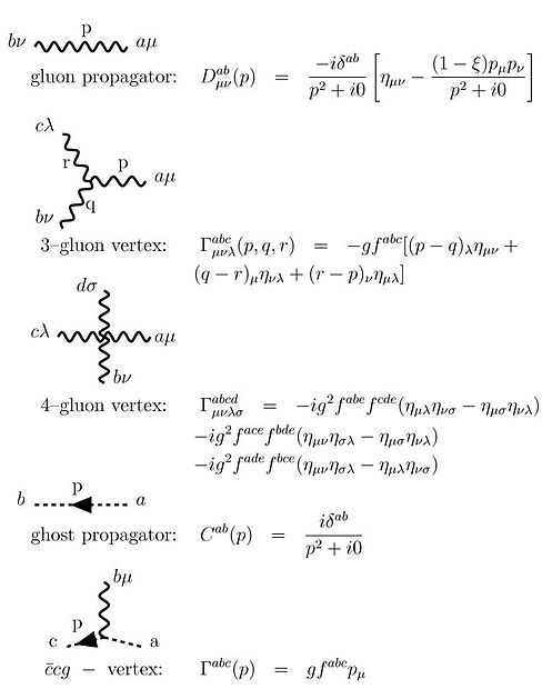
These rules for Feynman diagrams can be obtained when the generating functional given above is rewritten as
- Z[j,ε¯,ε]=exp(−ig∫d4xδiδε¯a(x)fabc∂μiδδjμb(x)iδδεc(x))×exp(−ig∫d4xfabc∂μiδδjνa(x)iδδjμb(x)iδδjcν(x))×exp(−ig24∫d4xfabcfarsiδδjμb(x)iδδjνc(x)iδδjrμ(x)iδδjsν(x))×Z0[j,ε¯,ε]{displaystyle {begin{aligned}Z[j,{bar {varepsilon }},varepsilon ]&=exp left(-igint d^{4}x,{frac {delta }{idelta {bar {varepsilon }}^{a}(x)}}f^{abc}partial _{mu }{frac {idelta }{delta j_{mu }^{b}(x)}}{frac {idelta }{delta varepsilon ^{c}(x)}}right)\&qquad times exp left(-igint d^{4}xf^{abc}partial _{mu }{frac {idelta }{delta j_{nu }^{a}(x)}}{frac {idelta }{delta j_{mu }^{b}(x)}}{frac {idelta }{delta j^{cnu }(x)}}right)\&qquad qquad times exp left(-i{frac {g^{2}}{4}}int d^{4}xf^{abc}f^{ars}{frac {idelta }{delta j_{mu }^{b}(x)}}{frac {idelta }{delta j_{nu }^{c}(x)}}{frac {idelta }{delta j^{rmu }(x)}}{frac {idelta }{delta j^{snu }(x)}}right)\&qquad qquad qquad times Z_{0}[j,{bar {varepsilon }},varepsilon ]end{aligned}}}
![{begin{aligned}Z[j,{bar {varepsilon }},varepsilon ]&=exp left(-igint d^{4}x,{frac {delta }{idelta {bar {varepsilon }}^{a}(x)}}f^{abc}partial _{mu }{frac {idelta }{delta j_{mu }^{b}(x)}}{frac {idelta }{delta varepsilon ^{c}(x)}}right)\&qquad times exp left(-igint d^{4}xf^{abc}partial _{mu }{frac {idelta }{delta j_{nu }^{a}(x)}}{frac {idelta }{delta j_{mu }^{b}(x)}}{frac {idelta }{delta j^{cnu }(x)}}right)\&qquad qquad times exp left(-i{frac {g^{2}}{4}}int d^{4}xf^{abc}f^{ars}{frac {idelta }{delta j_{mu }^{b}(x)}}{frac {idelta }{delta j_{nu }^{c}(x)}}{frac {idelta }{delta j^{rmu }(x)}}{frac {idelta }{delta j^{snu }(x)}}right)\&qquad qquad qquad times Z_{0}[j,{bar {varepsilon }},varepsilon ]end{aligned}}](https://wikimedia.org/api/rest_v1/media/math/render/svg/9c4cd58f4f16ab06d8fb1218150f659f5394cfbf)
with
- Z0[j,ε¯,ε]=exp(−∫d4xd4yε¯a(x)Cab(x−y)εb(y))exp(12∫d4xd4yjμa(x)Dabμν(x−y)jνb(y)){displaystyle Z_{0}[j,{bar {varepsilon }},varepsilon ]=exp left(-int d^{4}xd^{4}y{bar {varepsilon }}^{a}(x)C^{ab}(x-y)varepsilon ^{b}(y)right)exp left({tfrac {1}{2}}int d^{4}xd^{4}yj_{mu }^{a}(x)D^{abmu nu }(x-y)j_{nu }^{b}(y)right)}
![Z_{0}[j,{bar {varepsilon }},varepsilon ]=exp left(-int d^{4}xd^{4}y{bar {varepsilon }}^{a}(x)C^{ab}(x-y)varepsilon ^{b}(y)right)exp left({tfrac {1}{2}}int d^{4}xd^{4}yj_{mu }^{a}(x)D^{abmu nu }(x-y)j_{nu }^{b}(y)right)](https://wikimedia.org/api/rest_v1/media/math/render/svg/d337fe605a6ff373a5ec03cab3aae66197f40c04)
being the generating functional of the free theory. Expanding in g and computing the functional derivatives, we are able to obtain all the n-point functions with perturbation theory. Using LSZ reduction formula we get from the n-point functions the corresponding process amplitudes, cross sections and decay rates. The theory is renormalizable and corrections are finite at any order of perturbation theory.
For quantum electrodynamics the ghost field decouples because the gauge group is abelian. This can be seen from the coupling between the gauge field and the ghost field that is c¯afabc∂μAbμcc{displaystyle {bar {c}}^{a}f^{abc}partial _{mu }A^{bmu }c^{c}}

One of the most important results obtained for Yang–Mills theory is asymptotic freedom. This result can be obtained by assuming that the coupling constant g is small (so small nonlinearities), as for high energies, and applying perturbation theory. The relevance of this result is due to the fact that a Yang–Mills theory that describes strong interaction and asymptotic freedom permits proper treatment of experimental results coming from deep inelastic scattering.
To obtain the behavior of the Yang–Mills theory at high energies, and so to prove asymptotic freedom, one applies perturbation theory assuming a small coupling. This is verified a posteriori in the ultraviolet limit. In the opposite limit, the infrared limit, the situation is the opposite, as the coupling is too large for perturbation theory to be reliable. Most of the difficulties that research meets is just managing the theory at low energies. That is the interesting case, being inherent to the description of hadronic matter and, more generally, to all the observed bound states of gluons and quarks and their confinement (see hadrons). The most used method to study the theory in this limit is to try to solve it on computers (see lattice gauge theory). In this case, large computational resources are needed to be sure the correct limit of infinite volume (smaller lattice spacing) is obtained. This is the limit the results must be compared with. Smaller spacing and larger coupling are not independent of each other, and larger computational resources are needed for each. As of today, the situation appears somewhat satisfactory for the hadronic spectrum and the computation of the gluon and ghost propagators, but the glueball and hybrids spectra are yet a questioned matter in view of the experimental observation of such exotic states. Indeed, the σ resonance[6][7] is not seen in any of such lattice computations and contrasting interpretations have been put forward. This is a hotly debated issue.
Open problems
Yang–Mills theories met with general acceptance in the physics community after Gerard 't Hooft, in 1972, worked out their renormalization, relying on a formulation of the problem worked out by his advisor Martinus Veltman. (Their work[8] was recognized by the 1999 Nobel prize in physics.) Renormalizability is obtained even if the gauge bosons described by this theory are massive, as in the electroweak theory, provided the mass is only an "acquired" one, generated by the Higgs mechanism.
The mathematics of the Yang–Mills theory is a very active field of research, yielding e.g. invariants of differentiable structures on four-dimensional manifolds via work of Simon Donaldson. Furthermore, the field of Yang–Mills theories was included in the Clay Mathematics Institute's list of "Millennium Prize Problems". Here the prize-problem consists, especially, in a proof of the conjecture that the lowest excitations of a pure Yang–Mills theory (i.e. without matter fields) have a finite mass-gap with regard to the vacuum state. Another open problem, connected with this conjecture, is a proof of the confinement property in the presence of additional Fermion particles.
In physics the survey of Yang–Mills theories does not usually start from perturbation analysis or analytical methods, but more recently from systematic application of numerical methods to lattice gauge theories.
See also
- Aharonov–Bohm effect
- Coulomb gauge
- Electroweak theory
- Gauge covariant derivative
- Kaluza–Klein theory
- Lattice gauge theory
- Lorenz gauge
N = 4 supersymmetric Yang–Mills theory- Propagator
- Quantum chromodynamics
- Quantum gauge theory
- Field theoretical formulation of the standard model
- Symmetry in physics
- Weyl gauge
- Yang–Mills existence and mass gap
- Yang–Mills–Higgs equations
References
^ ab Straumann, N (2000). "On Pauli's invention of non-abelian Kaluza-Klein Theory in 1953". arXiv:gr-qc/0012054..mw-parser-output cite.citation{font-style:inherit}.mw-parser-output .citation q{quotes:"""""""'""'"}.mw-parser-output .citation .cs1-lock-free a{background:url("//upload.wikimedia.org/wikipedia/commons/thumb/6/65/Lock-green.svg/9px-Lock-green.svg.png")no-repeat;background-position:right .1em center}.mw-parser-output .citation .cs1-lock-limited a,.mw-parser-output .citation .cs1-lock-registration a{background:url("//upload.wikimedia.org/wikipedia/commons/thumb/d/d6/Lock-gray-alt-2.svg/9px-Lock-gray-alt-2.svg.png")no-repeat;background-position:right .1em center}.mw-parser-output .citation .cs1-lock-subscription a{background:url("//upload.wikimedia.org/wikipedia/commons/thumb/a/aa/Lock-red-alt-2.svg/9px-Lock-red-alt-2.svg.png")no-repeat;background-position:right .1em center}.mw-parser-output .cs1-subscription,.mw-parser-output .cs1-registration{color:#555}.mw-parser-output .cs1-subscription span,.mw-parser-output .cs1-registration span{border-bottom:1px dotted;cursor:help}.mw-parser-output .cs1-ws-icon a{background:url("//upload.wikimedia.org/wikipedia/commons/thumb/4/4c/Wikisource-logo.svg/12px-Wikisource-logo.svg.png")no-repeat;background-position:right .1em center}.mw-parser-output code.cs1-code{color:inherit;background:inherit;border:inherit;padding:inherit}.mw-parser-output .cs1-hidden-error{display:none;font-size:100%}.mw-parser-output .cs1-visible-error{font-size:100%}.mw-parser-output .cs1-maint{display:none;color:#33aa33;margin-left:0.3em}.mw-parser-output .cs1-subscription,.mw-parser-output .cs1-registration,.mw-parser-output .cs1-format{font-size:95%}.mw-parser-output .cs1-kern-left,.mw-parser-output .cs1-kern-wl-left{padding-left:0.2em}.mw-parser-output .cs1-kern-right,.mw-parser-output .cs1-kern-wl-right{padding-right:0.2em}
^ See Abraham Pais' account of this period as well as L. Susskind's "Superstrings, Physics World on the first non-abelian gauge theory" where Susskind wrote that Yang–Mills was "rediscovered" only because Pauli had chosen not to publish.
^ Reifler, N (2007). "Conditions for exact equivalence of Kaluza-Klein and Yang–Mills theories". arXiv:0707.3790.
^ Yang, C. N.; Mills, R. (1954). "Conservation of Isotopic Spin and Isotopic Gauge Invariance". Physical Review. 96 (1): 191–195. Bibcode:1954PhRv...96..191Y. doi:10.1103/PhysRev.96.191.
^ An Anecdote by C. N. Yang
^ Caprini, I.; Colangelo, G.; Leutwyler, H. (2006). "Mass and width of the lowest resonance in QCD". Physical Review Letters. 96 (13): 132001. arXiv:hep-ph/0512364. Bibcode:2006PhRvL..96m2001C. doi:10.1103/PhysRevLett.96.132001. PMID 16711979.
^ Yndurain, F. J.; Garcia-Martin, R.; Pelaez, J. R. (2007). "Experimental status of the ππ isoscalar S wave at low energy: f0(600) pole and scattering length". Physical Review D. 76 (7): 074034. arXiv:hep-ph/0701025. Bibcode:2007PhRvD..76g4034G. doi:10.1103/PhysRevD.76.074034.
^ 't Hooft, G.; Veltman, M. (1972). "Regularization and renormalization of gauge fields". Nuclear Physics B. 44: 189. Bibcode:1972NuPhB..44..189T. doi:10.1016/0550-3213(72)90279-9.
Further reading
- Books
Frampton, P. (2008). Gauge Field Theories (3rd ed.). Wiley-VCH. ISBN 978-3-527-40835-1.
Cheng, T.-P.; Li, L.-F. (1983). Gauge Theory of Elementary Particle Physics. Oxford University Press. ISBN 0-19-851961-3.
't Hooft, Gerardus (2005). 50 Years of Yang–Mills theory. World Scientific. ISBN 981-238-934-2.
- Articles
Svetlichny, George (1999). "Preparation for Gauge Theory". arXiv:math-ph/9902027.
Gross, D. (1992). "Gauge theory – Past, Present and Future". Retrieved 2015-05-05.
External links
| Wikiquote has quotations related to: Yang–Mills theory |
Hazewinkel, Michiel, ed. (2001) [1994], "Yang-Mills field", Encyclopedia of Mathematics, Springer Science+Business Media B.V. / Kluwer Academic Publishers, ISBN 978-1-55608-010-4
- Yang–Mills theory on DispersiveWiki
- The Clay Mathematics Institute
- The Millennium Prize Problems


